BORE: Bayesian Optimization by Density-Ratio Estimation

Bayesian Optimization (BO) by Density-Ratio Estimation (DRE), or BORE, is a simple, yet effective framework for the optimization of blackbox functions. BORE is built upon the correspondence between expected improvement (EI)—arguably the predominant acquisition functions used in BO—and the density-ratio between two unknown distributions.

One of the far-reaching consequences of this correspondence is that we can reduce the computation of EI to a probabilistic classification problem—a problem we are well-equipped to tackle, as evidenced by the broad range of streamlined, easy-to-use and, perhaps most importantly, battle-tested tools and frameworks available at our disposal for applying a variety of approaches. Notable among these are Keras / TensorFlow and PyTorch Lightning / PyTorch for Deep Learning, XGBoost for Gradient Tree Boosting, not to mention scikit-learn for just about everything else. The BORE framework lets us take direct advantage of these tools.

Code Example

We provide an simple example with Keras to give you a taste of how BORE can be implemented using a feed-forward neural network (NN) classifier. A useful class that the bore package provides is MaximizableSequential, a subclass of Sequential from Keras that inherits all of its existing functionalities, and provides just one additional method. We can build and compile a feed-forward NN classifier as usual:

from bore.models import MaximizableSequential
from tensorflow.keras.layers import Dense

# build model
classifier = MaximizableSequential()
classifier.add(Dense(16, activation="relu"))
classifier.add(Dense(16, activation="relu"))
classifier.add(Dense(1, activation="sigmoid"))

# compile model
classifier.compile(optimizer="adam", loss="binary_crossentropy")

See First contact with Keras from the Keras documentation if this seems unfamiliar to you.

The additional method provided is argmax, which returns the maximizer of the network, i.e. the input $\mathbf{x}$ that maximizes the final output of the network:

x_argmax = classifier.argmax(bounds=bounds, method="L-BFGS-B", num_start_points=3)

Since the network is differentiable end-to-end wrt to input $\mathbf{x}$, this method can be implemented efficiently using a multi-started quasi-Newton hill-climber such as L-BFGS. We will see the pivotal role this method plays in the next section.

Using this classifier, the BO loop in BORE looks as follows:

import numpy as np

features = []
targets = []

# initialize design
features.extend(features_initial_design)
targets.extend(targets_initial_design)

for i in range(num_iterations):

    # construct classification problem
    X = np.vstack(features)
    y = np.hstack(targets)

    tau = np.quantile(y, q=0.25)
    z = np.less(y, tau)

    # update classifier
    classifier.fit(X, z, epochs=200, batch_size=64)

    # suggest new candidate
    x_next = classifier.argmax(bounds=bounds, method="L-BFGS-B", num_start_points=3)

    # evaluate blackbox
    y_next = blackbox.evaluate(x_next)

    # update dataset
    features.append(x_next)
    targets.append(y_next)

Let’s break this down a bit:

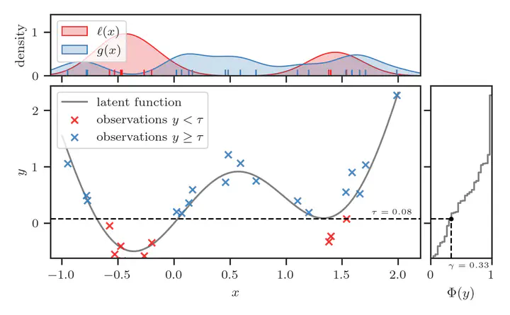
1. At the start of the loop, we construct the classification problem—by labeling instances $\mathbf{x}$ whose corresponding target value $y$ is in the top q=0.25 quantile of all target values as positive, and the rest as negative.

2. Next, we train the classifier to discriminate between these instances. This classifier should converge towards $${\pi }^{\ast }(\mathbf{x})=\frac{\gamma \ell (\mathbf{x})}{\gamma \ell (\mathbf{x})+(1-\gamma )g(\mathbf{x})},$$ where $\ell (\mathbf{x})$ and $g(\mathbf{x})$ are the unknown distributions of instances belonging to the positive and negative classes, respectively, and $\gamma$ is the class balance-rate and, by construction, simply the quantile we specified (i.e. $\gamma =0.25$).

3. Once the classifier is a decent approximation to ${\pi }^{\ast }(\mathbf{x})$, we propose the maximizer of this classifier as the next input to evaluate. In other words, we are now using the classifier itself as the acquisition function.

   How is it justifiable to use this in lieu of EI, or some other acquisition function we’re used to? And what is so special about ${\pi }^{\ast }(\mathbf{x})$?

   Well, as it turns out, ${\pi }^{\ast }(\mathbf{x})$ is equivalent to EI, up to some constant factors.

   The remainder of the loop should now be self-explanatory. Namely, we

4. evaluate the blackbox function at the suggested point, and

5. update the dataset.

Step-by-step Illustration

Here is a step-by-step animation of six iterations of this loop in action, using the Forrester synthetic function as an example. The noise-free function is shown as the solid gray curve in the main pane. This procedure is warm-started with four random initial designs.

The right pane shows the empirical CDF (ECDF) of the observed $y$ values. The vertical dashed black line in this pane is located at $\mathrm{\Phi }(y)=\gamma$, where $\gamma =0.25$. The horizontal dashed black line is located at $\tau$, the value of $y$ such that $\mathrm{\Phi }(y)=0.25$, i.e. $\tau ={\mathrm{\Phi }}^{-1}(0.25)$.

The instances below this horizontal line are assigned binary label $z=1$, while those above are assigned $z=0$. This is visualized in the bottom pane, alongside the probabilistic classifier ${\pi }_{\mathit{\theta }}(\mathbf{x})$ represented by the solid gray curve, which is trained to discriminate between these instances.

Finally, the maximizer of the classifier is represented by the vertical solid green line. This is the location at which the BO procedure suggests be evaluated next.

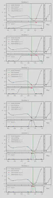
We see that the procedure converges toward to global minimum of the blackbox function after half a dozen iterations.

To understand how and why this works in more detail, please read our paper! If you only have 15 minutes to spare, please watch the video recording of our talk!

Video