A Primer on Pólya-gamma Random Variables - Part II: Bayesian Logistic Regression
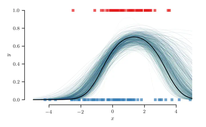
Table of Contents
Binary Classification
Consider the usual set-up for a binary classification problem:
for some input
Model – Bayesian Logistic Regression
Recall the standard Bayesian logistic regression model:
Likelihood
Let
Prior
For the sake of generality we discuss both the weight-space
and function-space views of Bayesian logistic regression.
In both cases, we consider a prior distribution in the form of a
multivariate Gaussian
Weight-space
In the weight-space view, sometimes referred to as linear logistic
regression, we assume a priori that the latent function takes the form
Function-space
In the function-space view, we assume the function is distributed according
to a Gaussian process (GP) with mean function
Inference and Prediction
Given some test input
Specifically, we first marginalize out the uncertainty about the associated
latent function value
But herein lies the real difficulty: the predictive
To overcome this intractability, one must typically resort to approximate inference methods such as the Laplace approximation1, variational inference (VI)2, expectation propagation (EP)3 and sampling-based approximations such as Markov Chain Monte Carlo (MCMC).
Augmented Model
Instead of appealing to approximate inference methods, let us consider an augmentation strategy that works by introducing auxiliary variables to the model4.
In particular, we introduce auxiliary variables
- Marginalizing out
- A Gaussian prior
Likelihood conditioned on auxiliary variables
First, let us define a conditional likelihood that factorize as
Prior over auxiliary variables
Second, let us define a prior over auxiliary variables
Pólya-gamma density (Polson et al. 2013)
A random variable
Property I: Recovering the original model
First we show that we can recover the original likelihood
Laplace transform of the Pólya-gamma density (Polson et al. 2013)
Based on the Laplace transform
of the Pólya-gamma density function, we can derive the following relationship:
Therefore, by substituting
Property II: Gaussian-Gaussian conjugacy
Let us define the diagonal matrix
Inference (Gibbs sampling)
We wish to compute the posterior
distribution
Each step of the Gibbs sampling procedure involves replacing the value of one
of the variables by a value drawn from the distribution of that variable
conditioned on the values of the remaining variables.
Specifically, we proceed as follows.
At step
- We first replace
- Then we replace
We then proceed in like manner, cycling between the two variables in turn until some convergence criterion is met.
Suffice it to say, this requires us to first compute the conditional
posteriors
Posterior over latent function values
The posterior over the latent function values
We readily obtain
Marginal and Conditional Gaussians (Bishop, Section 2.3.3, pg. 93)
Given a marginal Gaussian distribution for
Note that we also could have derived this directly without resorting to
the formulae above by reducing the product of two exponential-quadratic
functions in
Example: Gaussian process prior
To make this more concrete, let us revisit the Gaussian process prior we
discussed earlier, namely,
Posterior over auxiliary variables
The posterior over the auxiliary latent variables
Implementation (Weight-space view)
Having presented the general form of an augmented model for Bayesian logistic regression, we now derive a simple instance of this model to tackle a synthetic one-dimensional classification problem. In this particular implementation, we make the following choices: (a) we incorporate a basis function to project inputs into a higher-dimensional feature space, and (b) we consider an isotropic Gaussian prior on the weights.
Synthetic one-dimensional classification problem
First we synthesize a one-dimensional classification problem for which
the true class-membership probability
In code we can specify these as:
from scipy.stats import norm

p = norm(loc=1.0, scale=1.0)
q = norm(loc=0.0, scale=2.0)
We evenly draw a total of
>>> X_p, X_q = draw_samples(num_train, p, q, rate=0.5, random_state=random_state)
where the function draw_samples is defined as:
def draw_samples(num_samples, p, q, rate=0.5, random_state=None):

    num_top = int(num_samples * rate)
    num_bot = num_samples - num_top

    X_top = p.rvs(size=num_top, random_state=random_state)
    X_bot = q.rvs(size=num_bot, random_state=random_state)

    return X_top, X_bot
The densities of both distributions and their and samples are shown in the figure below.
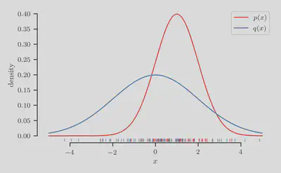
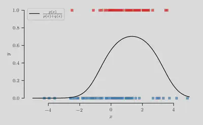
From these samples, let us now construct a classification dataset by assigning
label
>>> X_train, y_train = make_dataset(X_p, X_q)
where the function make_dataset is defined as:
def make_dataset(X_pos, X_neg):

    X = np.expand_dim(np.hstack([X_pos, X_neg]), axis=-1)
    y = np.hstack([np.ones_like(X_pos), np.zeros_like(X_neg)])

    return X, y
Crucially, the true class-membership probability is given exactly by
The class-membership probability
Prior
To increase the flexibility of our model, we introduce a basis
function
Therefore, we call:
>>> Phi = basis_function(X_train, degree=degree)
where the function basis_function is defined as:
def basis_function(x, degree=3):
    return np.power(x, np.arange(degree))
Let us define
the prior over weights as a simple isotropic Gaussian with
precision
m = np.zeros(latent_dim)

alpha = 2.0  # prior precision
S_inv = np.eye(latent_dim) / alpha

# initialize `beta`
beta = random_state.multivariate_normal(mean=m, cov=S_inv)
or more simply:
alpha = 2.0  # prior precision

# initialize `beta`
beta = random_state.normal(size=latent_dim, scale=1/np.sqrt(alpha))
Conditional likelihood
The conditional likelihood is defined like before, except we instead
condition on weights
Inference and Prediction
Posterior over latent function values
The posterior over the latent weights
Let us implement the function that computes the mean and covariance
of
def conditional_posterior_weights(Phi, kappa, alpha, omega):

    latent_dim = Phi.shape[-1]

    Sigma_inv = (omega * Phi.T) @ Phi + alpha * np.eye(latent_dim)

    mu = np.linalg.solve(Sigma_inv, Phi.T @ kappa)
    Sigma = np.linalg.solve(Sigma_inv, np.eye(latent_dim))

    return mu, Sigma
and a function to return samples from the multivariate Gaussian parameterized by this mean and covariance:
def gassian_sample(mean, cov, random_state=None):
    random_state = check_random_state(random_state)
    return random_state.multivariate_normal(mean=mean, cov=cov)
Posterior over auxiliary variables
The conditional posterior over the local auxiliary variable
Let us implement a function to compute the parameters of the posterior Polya-gamma distribution:
def conditional_posterior_auxiliary(Phi, beta):
    c = Phi @ beta
    b = np.ones_like(c)
    return b, c
and accordingly a function to return samples from this distribution:
def polya_gamma_sample(b, c, pg=PyPolyaGamma()):
    assert b.shape == c.shape, "shape mismatch"
    omega = np.empty_like(b)
    pg.pgdrawv(b, c, omega)
    return omega
where we have imported the PyPolyaGamma object from
the pypolyagamma package:
from pypolyagamma import PyPolyaGamma
The pypolyagamma package can be installed via pip as usual:
$ pip install pypolyagamma
To provide some context, this package is a Cython port, created by S. Linderman, of the original R package BayesLogit authored by J. Windle that implements the method described in their paper on the efficient sampling of Pólya-gamma variables6.
Gibbs sampling
With these functions defined, we can define the Gibbs sampling procedure by the simple for-loop below:
# preprocessing
kappa = y_train - 0.5
Phi = basis_function(X_train, degree=degree)

# initialize `beta`
latent_dim = Phi.shape[-1]
beta = random_state.normal(size=latent_dim, scale=1/np.sqrt(alpha))

for i in range(num_iterations):

    b, c = conditional_posterior_auxiliary(Phi, beta)
    omega = polya_gamma_sample(b, c, pg=pg)

    mu, Sigma = conditional_posterior_weights(Phi, kappa, alpha, omega)
    beta = gassian_sample(mu, Sigma, random_state=random_state)
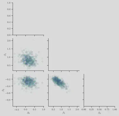
We now visualize the samples
First, we show the sampled weight vector
Second, we show the sampled auxiliary latent variables
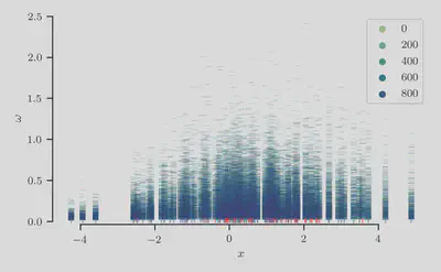
As expected, we find longer-tailed distributions in the variables
Finally, we plot the sampled class-membership probability predictions
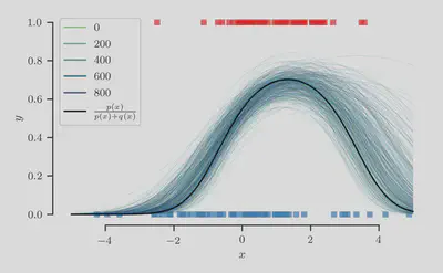
At least qualitatively, we find that the sampling procedure produces predictions that fit the true class-membership probability reasonably well.
Code
The full code is reproduced below:
import numpy as np

from scipy.stats import norm
from pypolyagamma import PyPolyaGamma

from .utils import (draw_samples, make_dataset, basis_function,
                    conditional_posterior_auxiliary, polya_gamma_sample,
                    conditional_posterior_weights, gassian_sample)

# constants
num_train = 128
num_iterations = 1000
degree = 3
alpha = 2.0  # prior precision

seed = 8888
random_state = np.random.RandomState(seed)
pg = PyPolyaGamma(seed=seed)

# generate dataset
p = norm(loc=1.0, scale=1.0)
q = norm(loc=0.0, scale=2.0)

X_p, X_q = draw_samples(num_train, p, q, rate=0.5, random_state=random_state)
X_train, y_train = make_dataset(X_p, X_q)

# preprocessing
kappa = y_train - 0.5
Phi = basis_function(X_train, degree=degree)

# initialize `beta`
latent_dim = Phi.shape[-1]
beta = random_state.normal(size=latent_dim, scale=1/np.sqrt(alpha))

for i in range(num_iterations):

    b, c = conditional_posterior_auxiliary(Phi, beta)
    omega = polya_gamma_sample(b, c, pg=pg)

    mu, Sigma = conditional_posterior_weights(Phi, kappa, alpha, omega)
    beta = gassian_sample(mu, Sigma, random_state=random_state)
where the module utils.py contains:
import numpy as np
from sklearn.utils import check_random_state
from pypolyagamma import PyPolyaGamma


def draw_samples(num_samples, p, q, rate=0.5, random_state=None):
    num_top = int(num_samples * rate)
    num_bot = num_samples - num_top

    X_top = p.rvs(size=num_top, random_state=random_state)
    X_bot = q.rvs(size=num_bot, random_state=random_state)
    return X_top, X_bot


def make_dataset(X_pos, X_neg):
    X = np.expand_dims(np.hstack([X_pos, X_neg]), axis=-1)
    y = np.hstack([np.ones_like(X_pos), np.zeros_like(X_neg)])
    return X, y


def basis_function(x, degree=3):
    return np.power(x, np.arange(degree))


def polya_gamma_sample(b, c, pg=PyPolyaGamma()):
    assert b.shape == c.shape, "shape mismatch"
    omega = np.empty_like(b)
    pg.pgdrawv(b, c, omega)
    return omega


def gassian_sample(mean, cov, random_state=None):
    random_state = check_random_state(random_state)
    return random_state.multivariate_normal(mean=mean, cov=cov)


def conditional_posterior_weights(Phi, kappa, alpha, omega):
    latent_dim = Phi.shape[-1]
    eye = np.eye(latent_dim)

    Sigma_inv = (omega * Phi.T) @ Phi + alpha * eye

    mu = np.linalg.solve(Sigma_inv, Phi.T @ kappa)
    Sigma = np.linalg.solve(Sigma_inv, eye)
    return mu, Sigma


def conditional_posterior_auxiliary(Phi, beta):
    c = Phi @ beta
    b = np.ones_like(c)
    return b, c
Bonus: Gibbs sampling with mutual recursion and generator delegation
The Gibbs sampling procedure naturally lends itself to implementations based
on mutual recursion.
Combining this with the yield from expression for generator delegation,
we can succinctly replace the for-loop with the following mutually recursive
functions:
def gibbs_sampler(beta, Phi, kappa, alpha, pg, random_state):
    b, c = conditional_posterior_auxiliary(Phi, beta)
    omega = polya_gamma_sample(b, c, pg=pg)
    yield from gibbs_sampler_helper(omega, Phi, kappa, alpha, pg, random_state)


def gibbs_sampler_helper(omega, Phi, kappa, alpha, pg, random_state):
    mu, Sigma = conditional_posterior_weights(Phi, kappa, alpha, omega)
    beta = gassian_sample(mu, Sigma, random_state=random_state)
    yield beta, omega
    yield from gibbs_sampler(beta, Phi, kappa, alpha, pg, random_state)
Now you can use gibbs_sampler as a generator,
for example, to explicitly iterate over it in a for-loop:
for beta, omega in gibbs_sampler(beta, Phi, kappa, alpha, pg, random_state):

    if stop_predicate:
        break

    # do something
    pass
or by making use of itertools and other functional programming primitives:
from itertools import islice

# example: collect beta and omega samples into respective lists
betas, omegas = zip(*islice(gibbs_sampler(beta, Phi, kappa, alpha, pg, random_state), num_iterations))
There are a few obvious drawbacks to this implementation. First, while it may be a lot fun to write, it will probably not be as fun to read when you revisit it later on down the line. Second, you may occasionally find yourself hitting the maximum recursion depth before you have reached a sufficient number of iterations for the warm-up or “burn-in” phase to have been completed. It goes without saying, the latter can make this implementation a non-starter.
Links and Further Readings
- Papers:
- Blog posts:
- Pólya-Gamma Augmentation by G. Gundersen
- Code:
- pypolyagamma: A Python package by S. Linderman
- BayesLogit: An R package by J. Windle
Cite as:
@article{tiao2021polyagamma,
  title   = "{A} {P}rimer on {P}ólya-gamma {R}andom {V}ariables - {P}art II: {B}ayesian {L}ogistic {R}egression",
  author  = "Tiao, Louis C",
  journal = "tiao.io",
  year    = "2021",
  url     = "https://tiao.io/post/polya-gamma-bayesian-logistic-regression/"
}
To receive updates on more posts like this, follow me on Twitter and GitHub!
Appendix
I
First, note that the logistic function can be written as
II
The conditional likelihood factorizes as
III
We have omitted the normalizing constant
Laplace transform of the
The Laplace transform
of the
Hence, by making the substitution
MacKay, D. J. (1992). The Evidence Framework Applied to Classification Networks. Neural Computation, 4(5), 720-736. ↩︎
Jaakkola, T. S., & Jordan, M. I. (2000). Bayesian Parameter Estimation via Variational Methods. Statistics and Computing, 10(1), 25-37. ↩︎
Minka, T. P. (2001, August). Expectation Propagation for Approximate Bayesian Inference. In Proceedings of the Seventeenth Conference on Uncertainty in Artificial Intelligence (pp. 362-369). ↩︎
Polson, N. G., Scott, J. G., & Windle, J. (2013). Bayesian Inference for Logistic Models using Pólya–Gamma Latent Variables. Journal of the American Statistical Association, 108(504), 1339-1349. ↩︎ ↩︎
Geman, S., & Geman, D. (1984). Stochastic Relaxation, Gibbs Distributions, and the Bayesian Restoration of Images. IEEE Transactions on Pattern Analysis and Machine Intelligence, (6), 721-741. ↩︎
Windle, J., Polson, N. G., & Scott, J. G. (2014). Sampling Pólya-gamma Random Variates: Alternate and Approximate Techniques. arXiv preprint arXiv:1405.0506. ↩︎
Wenzel, F., Galy-Fajou, T., Donner, C., Kloft, M., & Opper, M. (2019, July). Efficient Gaussian Process Classification using Pòlya-Gamma Data Augmentation. In Proceedings of the AAAI Conference on Artificial Intelligence (Vol. 33, No. 01, pp. 5417-5424). ↩︎
Snell, J., & Zemel, R. (2020). Bayesian Few-Shot Classification with One-vs-Each Pólya-Gamma Augmented Gaussian Processes. arXiv preprint arXiv:2007.10417. ↩︎