Fourier decomposition of Gaussian processes III

In a previous post, we explored how wavy lines claimed to be random functions drawn from a Gaussian process can be described as the sum of multiple sinusoidal waves. But how exactly is this useful for predictive modeling? 🔍

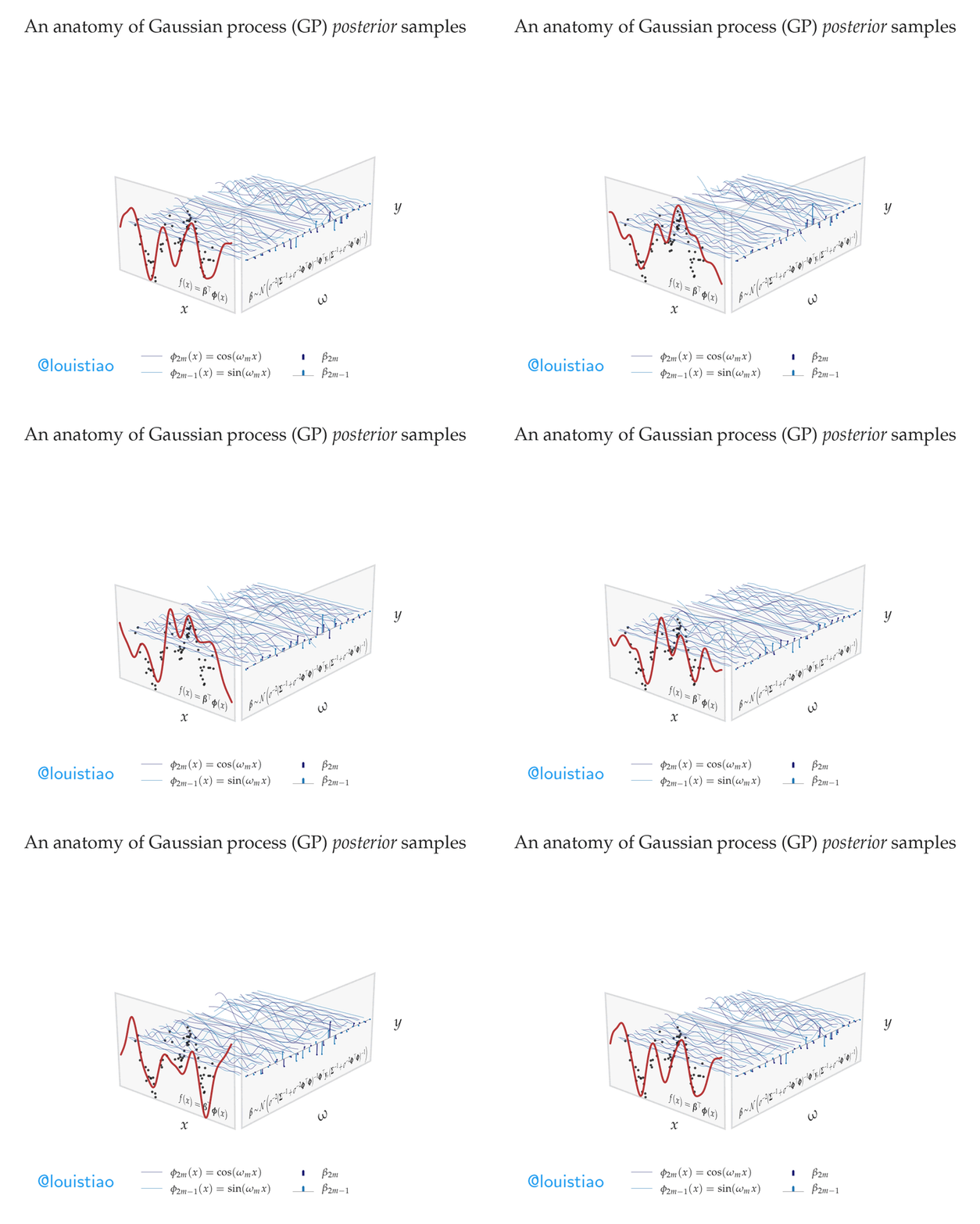
Suppose we were to use these sine waves as the basis functions in linear regression. Specifically, let’s model the target variable as a weighted sum of sine waves with different frequencies. Finding the best fit to the observed data then amounts to inferring suitable weights, or amplitudes, for each sinusoid. 📈

Assuming a Gaussian noise model, we can derive the posterior distribution over amplitudes – that is, the conditional distribution of the amplitudes given the observed data. We can draw samples from this posterior to make predictions. In this animation, we show predictions made using samples from the posterior smoothly transitioning between possible fits to the data. In fact, as before, these predictions can be viewed as random functions drawn from a Gaussian process, specifically, the posterior predictive process–a Gaussian process in itself! 🌟

Notably, the animation shows that amplitudes for many high-frequency sine waves are concentrated around fixed values, indicating low posterior uncertainty about the contribution of these rapidly varying basis functions. In contrast, amplitudes of lower frequencies oscillate more wildly, reflecting greater uncertainty about these smoother basis components. 🧠

This frequency-domain and weight-space perspective of Gaussian processes enables flexible nonlinear regression with inherent uncertainty quantification. The posterior captures our changing beliefs about the suitability of sine waves at different frequencies for explaining the data. ✨