An Illustrated Guide to the Knowledge Gradient Acquisition Function

We provide a short guide to the knowledge-gradient (KG) acquisition function (Frazier et al., 2009)¹ for Bayesian optimization (BO). Rather than being a self-contained tutorial, this posts is intended to serve as an illustrated compendium to the paper of Frazier et al., 2009¹ and the subsequent tutorial by Frazier, 2018², authored nearly a decade later.

This post assumes a basic level of familiarity with BO and Gaussian processes (GPs), to the extent provided by the literature survey of Shahriari et al., 2015³, and the acclaimed textbook of Rasmussen and Williams, 2006, respectively.

Knowledge-gradient

First, we set-up the notation and terminology. Let $f:\mathcal{X}\to \mathbb{R}$ be the blackbox function we wish to minimize. We denote the GP posterior predictive distribution, or predictive for short, by $p(y|\mathbf{x},\mathcal{D})$. The mean of the predictive, or the predictive mean for short, is denoted by $$\mu (\mathbf{x};\mathcal{D})=\mathbb{E}[y|\mathbf{x},\mathcal{D}]$$ Let ${\mathcal{D}}_n$ be the set of $n$ input-output observations ${\mathcal{D}}_n=\{({\mathbf{x}}_i,y_i){\}}_{i=1}^n$, where output $y_i=f({\mathbf{x}}_i)+ϵ$ is assumed to be observed with noise $ϵ\sim \mathcal{N}(0,{\sigma }^2)$. We make the following abbreviation $${\mu }_n(\mathbf{x})=\mu (\mathbf{x};{\mathcal{D}}_n)$$ Next, we define the minimum of the predictive mean, or predictive minimum for short, as $$\tau (\mathcal{D})=\underset{{\mathbf{x}}^{\prime }\in \mathcal{X}}{min}\mu ({\mathbf{x}}^{\prime };\mathcal{D})$$ If we view $\mu (\mathbf{x};\mathcal{D})$ as our fit to the underlying function $f(\mathbf{x})$ from which the observations $\mathcal{D}$ were generated, then $\tau (\mathcal{D})$ is our estimate of the minimum of $f(\mathbf{x})$, given observations $\mathcal{D}$.

Further, we make the following abbreviations $${\tau }_n=\tau ({\mathcal{D}}_n),\text{and}{\tau }_{n+1}=\tau ({\mathcal{D}}_{n+1}),$$ where ${\mathcal{D}}_{n+1}={\mathcal{D}}_n\cup \{(\mathbf{x},y)\}$ is the set of existing observations, augmented by some input-output pair $(\mathbf{x},y)$. Then, the knowledge-gradient is defined as $$\alpha (\mathbf{x};{\mathcal{D}}_n)={\mathbb{E}}_{p(y|\mathbf{x},{\mathcal{D}}_n)}[{\tau }_n-{\tau }_{n+1}]$$ Crucially, note that ${\tau }_{n+1}$ is implicitly a function of $(\mathbf{x},y)$, and that this expression integrates over all possible input-output observation pairs $(\mathbf{x},y)$ for the given $\mathbf{x}$ under the predictive $p(y|\mathbf{x},{\mathcal{D}}_n)$.

Monte Carlo estimation

Not surprisingly, the knowledge-gradient function is analytically intractable. Therefore, in practice, we compute it using Monte Carlo estimation, $$\alpha (\mathbf{x};{\mathcal{D}}_n)\approx \frac{1}{M}(\sum _{m=1}^M{\tau }_n-{\tau }_{n+1}^{(m)}),y^{(m)}\sim p(y|\mathbf{x},{\mathcal{D}}_n),$$ where ${\tau }_{n+1}^{(m)}=\tau ({\mathcal{D}}_{n+1}^{(m)})$ and ${\mathcal{D}}_{n+1}^{(m)}={\mathcal{D}}_n\cup \{(\mathbf{x},y^{(m)})\}$.

We refer to $y^{(m)}$ as the $m$th simulated outcome, or the $m$th simulation for short. Then, ${\mathcal{D}}_{n+1}^{(m)}$ is the $m$th simulation-augmented dataset and, accordingly, ${\tau }_{n+1}^{(m)}$ is the $m$th simulation-augmented predictive minimum.

We see that this approximation to the knowledge-gradient is simply the average difference between the predictive minimum values based on simulation-augmented data ${\tau }_{n+1}^{(m)}$, and that based on observed data ${\tau }_n$, across $M$ simulations.

This might take a moment to digest, as there are quite a number of moving parts to keep track of. To help visualize these parts, we provide an illustration of each of the steps required to compute KG on a simple one-dimensional synthetic problem.

One-dimensional example

As the running example throughout this post, we use a synthetic function defined as $$f(x)=\sin (3x)+x^2-0.7x.$$ We generate $n=10$ observations at locations sampled uniformly at random. The true function, and the set of noisy observations ${\mathcal{D}}_n$ are visualized in the figure below:

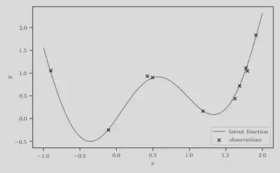
Using the observations ${\mathcal{D}}_n$ we have collected so far, we wish to use KG to score a candidate location $x_c$ at which to evaluate next.

Posterior predictive distribution

The posterior predictive $p(y|\mathbf{x},{\mathcal{D}}_n)$ is visualized in the figure below. In particular, the predictive mean ${\mu }_n(\mathbf{x})$ is represented by the solid orange curve.

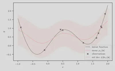
Clearly, this is a poor fit to the data and a uncalibrated estimation of the predictive uncertainly.

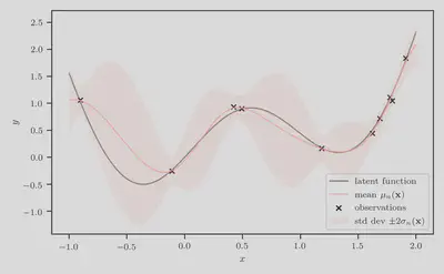
Step 1: Hyperparameter estimation

Therefore, first step is to optimize the hyperparameters of the GP regression model, i.e. the kernel lengthscale, amplitude, and the observation noise variance. We do this using type-II maximum likelihood estimation (MLE), or empirical Bayes.

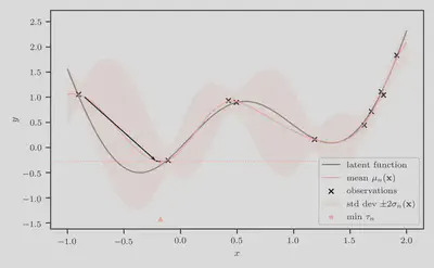
Step 2: Determine the predictive minimum

Next, we compute the predictive minimum ${\tau }_n=\underset{{\mathbf{x}}^{\prime }\in \mathcal{X}}{min}{\mu }_n({\mathbf{x}}^{\prime })$. Since ${\mu }_n$ is end-to-end differentiable wrt to input $\mathbf{x}$, we can simply use a multi-started quasi-Newton hill-climber such as L-BFGS. We visualize this in the figure below, where the value of the predictive minimum is represented by the orange horizontal dashed line, and its location is denoted by the orange star and triangle.

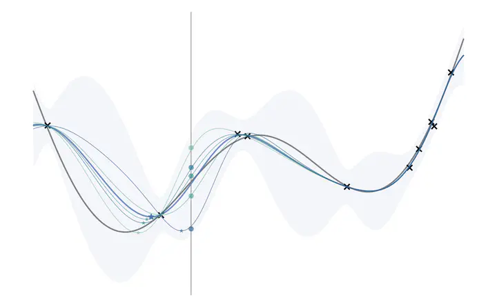
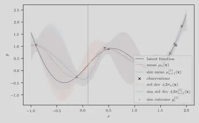
Step 3: Compute simulation-augmented predictive means

Suppose we are scoring the candidate location $x_c=0.1$. For illustrative purposes, let us draw just $M=1$ sample $y_c^{(1)}\sim p(y|x_c,{\mathcal{D}}_n)$. In the figure below, the candidate location $x_c$ is represented by the vertical solid gray line, and the single simulated outcome $y_c^{(1)}$ is represented by the filled blue dot.

In general, we denote the simulation-augmented predictive mean as $${\mu }_{n+1}^{(m)}(\mathbf{x})=\mu (\mathbf{x};{\mathcal{D}}_{n+1}^{(m)}),$$ where ${\mathcal{D}}_{n+1}^{(m)}={\mathcal{D}}_n\cup \{(\mathbf{x},y^{(m)})\}$ as defined earlier.

Here, the simulation-augmented dataset ${\mathcal{D}}_{n+1}^{(1)}$ is the set of existing observations ${\mathcal{D}}_n$, augmented by the simulated input-output pair $(x_c,y_c^{(1)})$, $${\mathcal{D}}_{n+1}^{(1)}={\mathcal{D}}_n\cup \{(x_c,y_c^{(1)})\},$$ and the corresponding simulation-augmented predictive mean ${\mu }_{n+1}^{(1)}(x)$ is represented in the figure below by the solid blue curve.

Step 4: Compute simulation-augmented predictive minimums

Next, we compute the simulation-augmented predictive minimum $${\tau }_{n+1}^{(1)}=\underset{{\mathbf{x}}^{\prime }\in \mathcal{X}}{min}{\mu }_{n+1}^{(1)}({\mathbf{x}}^{\prime })$$ It may not be immediately obvious, but ${\mu }_{n+1}^{(1)}$ is in fact also end-to-end differentiable wrt to input $\mathbf{x}$. Therefore, we can again appeal to an method such as L-BFGS. We visualize this in the figure below, where the value of the simulation-augmented predictive minimum is represented by the blue horizontal dashed line, and its location is denoted by the blue star and triangle.

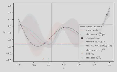
Taking the difference between the orange and blue horizontal dashed line will give us an unbiased estimate of the knowledge-gradient. However, this is likely to be a crude one, since it is based on just a single MC sample. To obtain a more accurate estimate, one needs to increase $M$, the number of MC samples.

Samples $M>1$

Let us now consider $M=5$ samples. We draw $y_c^{(m)}\sim p(y|x_c,{\mathcal{D}}_n)$, for $m=1,\dots ,5$. As before, the input location $x_c$ is represented by the vertical solid gray line, and the corresponding simulated outcomes are represented by the filled dots below, with varying hues from a perceptually uniform color palette to distinguish between samples.

Accordingly, the simulation-augmented predictive means ${\mu }_{n+1}^{(m)}(x)$ at location $x_c=0.1$, for $m=1,\dots ,5$ are represented by the colored curves, with hues set to that of the simulated outcome on which the predictive distribution is based.

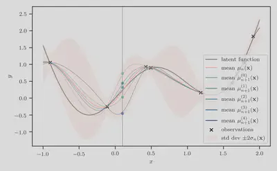
Next we compute the simulation-augmented predictive minimum ${\tau }_{n+1}^{(m)}$, which requires minimizing ${\mu }_{n+1}^{(m)}(x)$ for $m=1,\dots ,5$. These values are represented below by the horizontal dashed lines, and their location is denoted by the stars and triangles.

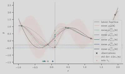
Finally, taking the average difference between the orange dashed line and every other dashed line gives us the estimate of the knowledge gradient at input $x_c$.

Links and Further Readings

• In this post, we only showed a (naïve) approach to calculating the KG at a given location. Suffice it to say, there is still quite a gap between this and being able to efficiently minimize KG within a sequential decision-making algorithm. For a guide on incorporating KG in a modular and fully-fledged framework for BO (namely BOTorch) see The One-shot Knowledge Gradient Acquisition Function
• Another introduction to KG: Expected Improvement vs. Knowledge Gradient

Cite as:

@article{tiao2021knowledge,
  title   = "{A}n {I}llustrated {G}uide to the {K}nowledge {G}radient {A}cquisition {F}unction",
  author  = "Tiao, Louis C",
  journal = "tiao.io",
  year    = "2021",
  url     = "https://tiao.io/post/an-illustrated-guide-to-the-knowledge-gradient-acquisition-function/"
}

To receive updates on more posts like this, follow me on Twitter and GitHub!