A Primer on Pólya-gamma Random Variables - Part III: Local Variational Methods

This is Part III of a three-part series on Pólya-Gamma random variables. See also: Part I — Basic Relationships and Part II — Bayesian Logistic Regression.
Table of Contents
In Part II we augmented Bayesian logistic regression with Pólya-gamma auxiliary variables and recovered conjugacy: conditioned on the auxiliary variables $\boldsymbol{\omega}$, the posterior over the latent function is Gaussian, and conditioned on the latent function, the posterior over each $\omega_n$ is again Pólya-gamma. Cycling between the two conditionals gave us a Gibbs sampler whose draws converge to the exact posterior.
Exact is a fine quality in a posterior, but sampling has its costs. The draws are correlated and sequential, convergence is something you diagnose rather than prove, and every prediction requires dragging a bag of samples around. The standard deterministic alternative is variational inference (VI): pick a family of tractable distributions, and find the member closest in KL divergence to the posterior by maximizing a lower bound on the marginal likelihood. In this post we do the most pedestrian thing available: mean-field VI in the same augmented model, turning the crank without a single clever idea.
The method that falls out is older than the Pólya-gamma distribution by some fifteen years. It is the local variational method of Jaakkola and Jordan1, a staple of the approximate inference literature (Bishop’s PRML devotes Section 10.6 to it2) built on a quadratic lower bound to the logistic log-likelihood with one free parameter $\xi_n$ per datapoint. Their bound, their mysteriously specific coefficient function $\lambda(\xi)$, and their EM-style updates all reappear here, one for one. The correspondence is exact rather than merely analogical, a point made precise by Durante and Rigon3.
Seen through the variational lens, three small mysteries of the classical derivation resolve themselves:
- the coefficient $\lambda(\xi)$ is the mean of a Pólya-gamma distribution;
- the local variational parameter $\xi_n$ parameterizes a Pólya-gamma variational factor $q(\omega_n)$, through exponential tilting;
- the slack in the bound is exactly a KL divergence, which is why the bound touches the sigmoid precisely at $\psi = \pm \xi$ and nowhere else.
None of this is visible from the classical derivation, which we will also revisit toward the end, where the bound is produced by a convexity argument and its tightness pattern looks like a happy accident of calculus.
The Augmented Model, Briefly
We work in the weight-space view with basis functions, which keeps us close to both the eventual implementation and the setting of Jaakkola and Jordan. Everything below goes through unchanged in the function-space view with $f_n$ in place of $\psi_n$ (see Part II).
For inputs $\mathbf{x}_n$ with binary targets $y_n \in \{0, 1\}$, let $\boldsymbol{\phi}_n = \phi(\mathbf{x}_n)$ be the feature vector of the $n$th input and let
$$ \psi_n \triangleq \boldsymbol{\beta}^{\top} \boldsymbol{\phi}_n $$be the corresponding value of the latent function. We place a Gaussian prior on the weights, written in terms of its precision matrix $\mathbf{S}$,
$$ p(\boldsymbol{\beta}) = \mathcal{N}(\boldsymbol{\beta} | \mathbf{m}, \mathbf{S}^{-1}), $$and, following Part II, we replace each Bernoulli likelihood factor with its augmented counterpart
$$ \begin{align*} p(y_n | \omega_n, \boldsymbol{\beta}) &= \frac{1}{2} \exp{\left\{-\frac{\omega_n}{2}\left(\psi_n^2 - 2\psi_n\frac{\kappa_n}{\omega_n}\right)\right\}} \newline &= \frac{1}{2} \exp{\left( \kappa_n \psi_n - \frac{\psi_n^2}{2} \omega_n \right)}, \end{align*} $$where $\kappa_n = y_n - \frac{1}{2}$, together with the Pólya-gamma prior
$$ p(\omega_n) = \mathrm{PG}(\omega_n | 1, 0). $$The model joint then factorizes as
$$ p(\mathbf{y}, \boldsymbol{\omega}, \boldsymbol{\beta}) = p(\boldsymbol{\beta}) \prod_{n=1}^N p(y_n | \omega_n, \boldsymbol{\beta}) p(\omega_n). $$Recall from Part II that marginalizing out the auxiliary variable recovers the original likelihood exactly,
$$ \begin{align*} p(y | \boldsymbol{\beta}) & = \int p(y | \omega, \boldsymbol{\beta}) p(\omega) \mathrm{d}\omega \newline & = \frac{e^{y \psi}}{1 + e^{\psi}} = \sigma(\psi)^{y} (1-\sigma(\psi))^{1-y} = \mathrm{Bern}(y | \sigma(\psi)), \end{align*} $$so the augmented model is the same model, wearing more convenient clothes.
In Part II we sampled from $p(\boldsymbol{\beta}, \boldsymbol{\omega} | \mathbf{y})$ by Gibbs sampling. Here we approximate it instead.
Mean-Field Variational Inference
We posit a variational distribution that factorizes between the weights and the auxiliary variables,
$$ q(\boldsymbol{\beta}, \boldsymbol{\omega}) = q(\boldsymbol{\beta}) \prod_{n=1}^N q(\omega_n; \xi_n), $$and maximize the evidence lower bound (ELBO)
$$ \log p(\mathbf{y}) \geq \mathcal{L}(q) \triangleq \mathbb{E}_{q(\boldsymbol{\beta}, \boldsymbol{\omega})} [\log p(\mathbf{y}, \boldsymbol{\omega}, \boldsymbol{\beta}) - \log q(\boldsymbol{\beta}, \boldsymbol{\omega})], $$which is equivalent to minimizing $\mathrm{KL}[q(\boldsymbol{\beta}, \boldsymbol{\omega}) \, \| \, p(\boldsymbol{\beta}, \boldsymbol{\omega} | \mathbf{y})]$.
For each auxiliary factor we adopt the family of exponentially tilted Pólya-gamma distributions with parameter $\xi_n$,
$$ \begin{align*} q(\omega_n; \xi_n) &\triangleq \mathrm{PG}(\omega_n | 1, \xi_n) \newline &= \cosh{\left(\frac{\xi_n}{2}\right)} \exp{\left(-\frac{\xi_n^2}{2}\omega_n\right)} \mathrm{PG}(\omega_n | 1, 0). \end{align*} $$This is not an arbitrary choice. Part II showed that the exact conditional posterior is $p(\omega_n | \psi_n) = \mathrm{PG}(1, \psi_n)$, so the family contains the distribution we are trying to approximate; and, as we will verify later, the optimal mean-field factor lands in this family whether we ask for it or not.
Two properties of the tilted family do all of the work in this post. The first is its mean.
The first moment of the Pólya-gamma distribution $\mathrm{PG}(\omega | b, c)$ is
$$ \mathbb{E}_{\mathrm{PG}(\omega | b, c)}[\omega] = \frac{b}{2c} \tanh{\left(\frac{c}{2}\right)} = b \cdot \lambda(c), \qquad \lambda(c) \triangleq \frac{1}{2c} \tanh{\left(\frac{c}{2}\right)}, $$so in particular $\mathbb{E}_{q(\omega; \xi)}[\omega] = \lambda(\xi)$.
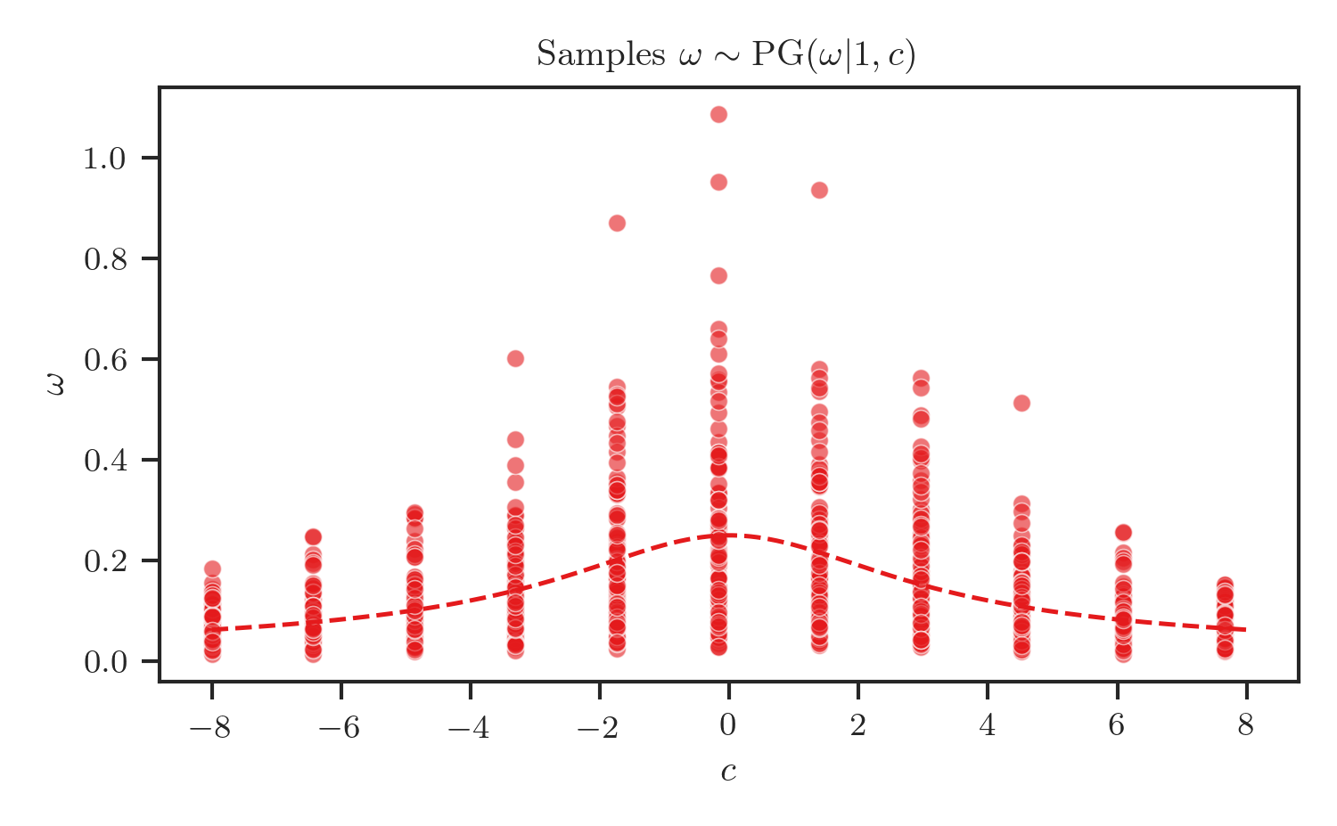
Samples $\omega \sim \mathrm{PG}(\omega | 1, c)$ with the mean function $\mathbb{E}[\omega] = \lambda(c)$ overlaid (dashed). Keep this function in mind; it is about to become famous.
The second is that the KL divergence from the tilted distribution to the prior is available in closed form, despite the Pólya-gamma density itself having no closed form. The log-ratio of the two densities is affine in $\omega$,
$$ \log \frac{q(\omega; \xi)}{p(\omega)} = \log{\cosh{\left(\frac{\xi}{2}\right)}} - \frac{\xi^2}{2}\omega, $$so taking the expectation under $q$ costs us nothing more than the first moment:
$$ \mathrm{KL}[q(\omega; \xi) \, \| \, p(\omega)] = \log{\cosh{\left(\frac{\xi}{2}\right)}} - \frac{\xi^2}{2} \lambda(\xi). $$Grinding Through the ELBO
Because the augmented likelihood factorizes across datapoints, the ELBO decomposes into per-datapoint contributions,
$$ \mathcal{L}(q) = \mathbb{E}_{q(\boldsymbol{\beta})} \left[ \sum_{n=1}^N H(y_n, \xi_n, \boldsymbol{\beta}) + \log{p(\boldsymbol{\beta})} - \log{q(\boldsymbol{\beta})} \right], $$where the per-datapoint term collects everything involving $\omega_n$,
$$ H(y, \xi, \boldsymbol{\beta}) \triangleq \mathbb{E}_{q(\omega;\xi)}[\log{p(y | \omega, \boldsymbol{\beta})}] - \mathrm{KL}[q(\omega;\xi) \, \| \, p(\omega)]. $$Let us compute it. Writing the augmented likelihood as $\log p(y | \omega, \boldsymbol{\beta}) = \kappa \psi - \frac{\psi^2}{2}\omega - \log 2$ and using the affine log-ratio from the previous section,
$$ \begin{align*} H(y, \xi, \boldsymbol{\beta}) &= \mathbb{E}_{q(\omega;\xi)}\left[\log{p(y | \omega, \boldsymbol{\beta})} + \log{p(\omega)} - \log{q(\omega;\xi)}\right] \newline &= \mathbb{E}_{q(\omega;\xi)} \left[ \kappa \psi - \frac{\psi^2}{2} \omega + \frac{\xi^2}{2} \omega \right] - \log{2} - \log{\cosh{\left(\frac{\xi}{2}\right)}} \newline &= \kappa \psi -\frac{\lambda(\xi)}{2} (\psi^2 - \xi^2) + \log{\sigma(\xi)} - \frac{\xi}{2}, \end{align*} $$where the last step uses $\mathbb{E}_{q(\omega;\xi)}[\omega] = \lambda(\xi)$ together with the identity $-\log{\left(2\cosh{\left(\frac{\xi}{2}\right)}\right)} = \log{\sigma(\xi)} - \frac{\xi}{2}$, which follows from Part I’s expression of the sigmoid in terms of the hyperbolic cosine. Substituting $\kappa = y - \frac{1}{2}$ gives
$$ H(y, \xi, \boldsymbol{\beta}) = y \psi - \frac{\psi + \xi}{2} -\frac{\lambda(\xi)}{2} (\psi^2 - \xi^2) + \log{\sigma(\xi)}. $$The ELBO thus replaces each exact log-likelihood term $\log p(y_n | \boldsymbol{\beta})$ with $H(y_n, \xi_n, \boldsymbol{\beta})$. It is worth staring at what we just built. Define
$$ \begin{align*} h(y, \xi, \boldsymbol{\beta}) &\triangleq \exp{H(y, \xi, \boldsymbol{\beta})} \newline &= \sigma(\xi) \exp{\left(y \psi - \frac{\psi + \xi}{2} - \frac{\lambda(\xi)}{2} (\psi^2 - \xi^2)\right)}. \end{align*} $$This is a pseudo-likelihood: a squashed-down stand-in for the Bernoulli factor, with the squashing controlled by $\xi$.
An Old Friend
Readers who have met variational logistic regression before will have recognized $h$ already. For everyone else, here is the classical result we have just rederived.
The Jaakkola-Jordan bound (Jaakkola and Jordan, 2000)
For any $\psi, \xi \in \mathbb{R}$,
$$ \begin{align*} \sigma(\psi) &\geq \ell(\psi, \xi) \triangleq \sigma(\xi) \exp{\left(\frac{\psi - \xi}{2} - \frac{\lambda(\xi)}{2} (\psi^2 - \xi^2)\right)}, \newline \lambda(\xi) &= \frac{1}{2\xi} \tanh{\left(\frac{\xi}{2}\right)}, \end{align*} $$with equality if and only if $\xi = \pm\psi$.
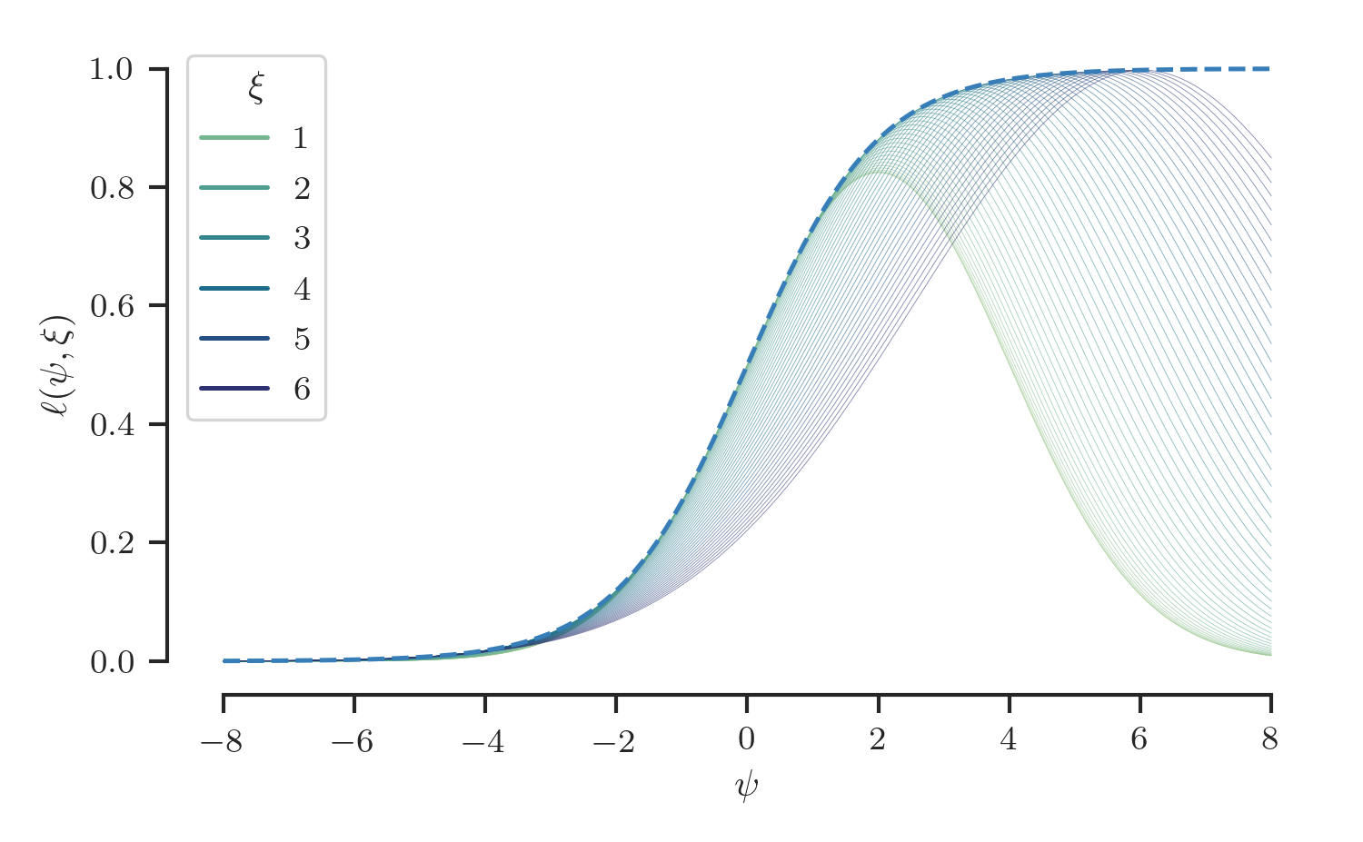
The logistic sigmoid function (dashed) and the family of Jaakkola-Jordan lower bounds $\ell(\psi, \xi)$, one curve per value of $\xi$. Each bound is exact at $\psi = \pm\xi$.
A line of algebra confirms that our per-datapoint pseudo-likelihood is exactly this bound, applied to the likelihood:
$$ h(y, \xi, \boldsymbol{\beta}) = e^{y\psi} \, \ell(-\psi, \xi) = \ell\left((2y - 1) \, \psi, \, \xi\right), $$which for $y = 1$ reads $\ell(\psi, \xi) \leq \sigma(\psi)$ and for $y = 0$ reads $\ell(-\psi, \xi) \leq \sigma(-\psi)$; in both cases, $h(y, \xi, \boldsymbol{\beta}) \leq p(y | \boldsymbol{\beta})$.
In other words: the mean-field ELBO of the Pólya-gamma augmented model is the Jaakkola-Jordan objective. Maximizing the ELBO over the variational parameters $\xi_n$ is the same computation as tightening the classical bounds; the “local variational parameter” attached to each datapoint is, from where we now stand, the tilting parameter of a Pólya-gamma variational factor $q(\omega_n) = \mathrm{PG}(1, \xi_n)$. And the coefficient $\lambda(\xi)$, which the classical derivation produces as the slope of a certain tangent line, is the posterior-mean function of the Pólya-gamma family — the dashed curve in Figure 1.4
One small observation while we are here: the Pólya-gamma density $\mathrm{PG}(1, \xi)$ depends on $\xi$ only through $\xi^2$, so $q(\omega; \xi)$ and $q(\omega; -\xi)$ are the same distribution. The classical bound’s indifference to the sign of $\xi$ stops being a curiosity; the two signs were never different objects to begin with.
The Slack in the Bound Is a KL Divergence
The variational view owes us one more explanation: why is the bound exact at $\xi = \pm\psi$, exactly there, and nowhere else?
For a fixed $\boldsymbol{\beta}$ (hence fixed $\psi$), the quantity $H(y, \xi, \boldsymbol{\beta})$ is itself a little ELBO for the one-dimensional latent variable $\omega$, and the generic ELBO identity applies: the gap to the true log-likelihood is the KL divergence from the variational factor to the exact conditional posterior. Part II computed that conditional: $p(\omega | y, \boldsymbol{\beta}) = \mathrm{PG}(1, \psi)$, independent of $y$. So
$$ \log{p(y | \boldsymbol{\beta})} - H(y, \xi, \boldsymbol{\beta}) = \mathrm{KL}[\, \mathrm{PG}(1, \xi) \, \| \, \mathrm{PG}(1, \psi) \,], $$and because both distributions are exponential tiltings of the same base measure, this KL divergence is available in closed form (see Appendix I):
$$ \begin{align*} & \mathrm{KL}[\, \mathrm{PG}(1, \xi) \, \| \, \mathrm{PG}(1, \psi) \,] = \newline & \qquad \log{\cosh{\left(\frac{\xi}{2}\right)}} - \log{\cosh{\left(\frac{\psi}{2}\right)}} + \frac{\psi^2 - \xi^2}{2} \lambda(\xi). \end{align*} $$Specializing to $y = 1$ gives a pleasingly compact form of the classical bound’s multiplicative slack:
$$ \frac{\sigma(\psi)}{\ell(\psi, \xi)} = \exp{\left( \mathrm{KL}[\, \mathrm{PG}(1, \xi) \, \| \, \mathrm{PG}(1, \psi) \,] \right)}. $$The right-hand side is $\geq 1$ because KL divergences are nonnegative (there is the bound), and it equals $1$ precisely when the two distributions coincide, that is, when $\xi = \pm\psi$ (there is the tightness pattern). What the classical derivation presents as an accident of tangency is the statement that a KL divergence vanishes exactly when its two arguments are equal.
These identities are checked numerically, to machine precision, by the
script verify_identities.py in this post’s source bundle.
Coordinate Ascent, and Why the Family Was Never a Choice
So far we fixed the form of $q(\omega_n)$ by fiat. Coordinate ascent variational inference (CAVI) lets us drop even that: holding the other factors fixed, the optimal mean-field factor for any block is the exponentiated expected log of the joint. For $\omega_n$,
$$ \begin{align*} q^*(\omega_n) &\propto p(\omega_n) \exp{\left( \mathbb{E}_{q(\boldsymbol{\beta})}[\log{p(y_n | \omega_n, \boldsymbol{\beta})}] \right)} \newline &\propto p(\omega_n) \exp{\left( - \frac{\mathbb{E}_{q(\boldsymbol{\beta})}[\psi_n^2]}{2} \omega_n \right)}, \end{align*} $$since the expected augmented log-likelihood is affine in $\omega_n$. An exponential tilting of $\mathrm{PG}(1, 0)$ is a Pólya-gamma distribution, so the optimum lands in our family automatically,
$$ q^*(\omega_n) = \mathrm{PG}(\omega_n | 1, \xi_n), \qquad \xi_n^2 = \mathbb{E}_{q(\boldsymbol{\beta})}[\psi_n^2] = \boldsymbol{\phi}_n^{\top} \left( \boldsymbol{\Sigma} + \boldsymbol{\mu} \boldsymbol{\mu}^{\top} \right) \boldsymbol{\phi}_n. $$The tilted family was never an assumption; it is forced by the model.
The optimal weight factor follows the same recipe. With $\boldsymbol{\Lambda} \triangleq \mathrm{diag}(\lambda(\xi_1), \dotsc, \lambda(\xi_N))$ collecting the expectations $\mathbb{E}_{q(\omega_n)}[\omega_n]$,
$$ \begin{align*} \log{q^*(\boldsymbol{\beta})} &= \log{p(\boldsymbol{\beta})} + \sum_{n=1}^N \mathbb{E}_{q(\omega_n)}[\log{p(y_n | \omega_n, \boldsymbol{\beta})}] + \mathrm{const} \newline &= -\frac{1}{2} (\boldsymbol{\beta} - \mathbf{m})^{\top} \mathbf{S} (\boldsymbol{\beta} - \mathbf{m}) \newline &\qquad + \sum_{n=1}^N \left( \kappa_n \psi_n - \frac{\lambda(\xi_n)}{2} \psi_n^2 \right) + \mathrm{const} \newline &= -\frac{1}{2} \boldsymbol{\beta}^{\top} \left(\mathbf{S} + \boldsymbol{\Phi}^{\top} \boldsymbol{\Lambda} \boldsymbol{\Phi}\right) \boldsymbol{\beta} + \boldsymbol{\beta}^{\top} \left(\mathbf{S} \mathbf{m} + \boldsymbol{\Phi}^{\top} \boldsymbol{\kappa} \right) + \mathrm{const}, \end{align*} $$which is the log of a Gaussian,
$$ \begin{align*} q^*(\boldsymbol{\beta}) &= \mathcal{N}(\boldsymbol{\beta} | \boldsymbol{\mu}, \boldsymbol{\Sigma}), \newline \boldsymbol{\mu} &= \boldsymbol{\Sigma} \left ( \mathbf{S} \mathbf{m} + \boldsymbol{\Phi}^{\top} \boldsymbol{\kappa} \right ), \qquad \boldsymbol{\Sigma} = \left( \mathbf{S} + \boldsymbol{\Phi}^{\top} \boldsymbol{\Lambda} \boldsymbol{\Phi} \right)^{-1}. \end{align*} $$CAVI alternates these two updates until convergence. Anyone who has implemented variational logistic regression from Bishop Section 10.6 will recognize both of them: the $q(\boldsymbol{\beta})$ update is Jaakkola and Jordan’s “E-step” and the $\xi$ update $\xi_n^2 = \mathbb{E}[\psi_n^2]$ is their “M-step”, derived there by maximizing the bound with respect to each $\xi_n$ directly. The two algorithms coincide, update for update. This is the equivalence formalized by Durante and Rigon3: Jaakkola and Jordan’s local variational method is mean-field variational Bayes in the Pólya-gamma augmented model, fifteen years avant la lettre.
The correspondence with Part II’s Gibbs sampler is equally mechanical:
| Gibbs (Part II) | CAVI (this post) | |
|---|---|---|
| $\omega$-step | draw $\omega_n \sim \mathrm{PG}(1, \psi_n)$ | set $q(\omega_n) = \mathrm{PG}(1, \xi_n)$, $\xi_n^2 = \mathbb{E}_q[\psi_n^2]$ |
| $\beta$-step | draw $\boldsymbol{\beta} \sim \mathcal{N}(\boldsymbol{\mu}_{\boldsymbol{\omega}}, \boldsymbol{\Sigma}_{\boldsymbol{\omega}})$, $\enspace \boldsymbol{\Sigma}_{\boldsymbol{\omega}} = \left( \mathbf{S} + \boldsymbol{\Phi}^{\top} \boldsymbol{\Omega} \boldsymbol{\Phi} \right)^{-1}$ | set $q(\boldsymbol{\beta}) = \mathcal{N}(\boldsymbol{\mu}, \boldsymbol{\Sigma})$, $\enspace \boldsymbol{\Sigma} = \left( \mathbf{S} + \boldsymbol{\Phi}^{\top} \boldsymbol{\Lambda} \boldsymbol{\Phi} \right)^{-1}$ |
Same two conditionals, with draws replaced by expectations: $\boldsymbol{\Lambda} = \mathbb{E}_q[\boldsymbol{\Omega}]$. Even the pseudo-observations survive the translation. Completing the square in $\psi$ shows that, up to constants in $\boldsymbol{\beta}$,
$$ h(y, \xi, \boldsymbol{\beta}) \propto \exp{\left\{-\frac{\lambda(\xi)}{2}\left(\psi - \frac{\kappa}{\lambda(\xi)}\right)^2\right\}}, $$a Gaussian pseudo-likelihood with precision $\lambda(\xi_n)$ and pseudo-target $\kappa_n / \lambda(\xi_n)$, where Part II had precision $\omega_n$ and pseudo-target $z_n = \kappa_n / \omega_n$.
One structural remark before we compute anything. In the exact posterior, the $\omega_n$ are already conditionally independent given $\boldsymbol{\beta}$, and our $q(\boldsymbol{\beta})$ is a full-covariance Gaussian. The only dependence the mean-field factorization severs is the one between $\boldsymbol{\beta}$ and $\boldsymbol{\omega}$. Whatever approximation error we observe below is attributable to that single cut.
Implementation
A pleasant consequence of trading Gibbs for CAVI is that the Pólya-gamma sampler, the one piece of specialized machinery Part II depended on, is no longer needed. The algorithm only ever touches $\boldsymbol{\omega}$ through the expectation $\lambda(\xi)$, which is one line of NumPy:
import numpy as np


def lambd(xi):
    return 0.5 * np.tanh(0.5 * xi) / xi
The entire inference algorithm is barely a dozen more. We alternate the two updates from the previous section, with the isotropic prior $\mathbf{m} = \mathbf{0}$, $\mathbf{S} = \alpha \mathbf{I}$ from Part II:
def cavi(Phi, kappa, alpha, num_iterations=200, tol=1e-12):

    latent_dim = Phi.shape[-1]
    eye = np.eye(latent_dim)

    xi = 1e-1 * np.ones(len(kappa))

    for _ in range(num_iterations):

        # update q(beta) = N(mu, Sigma), with Lambda = diag(lambd(xi))
        Sigma_inv = (lambd(xi) * Phi.T) @ Phi + alpha * eye
        mu = np.linalg.solve(Sigma_inv, Phi.T @ kappa)
        Sigma = np.linalg.solve(Sigma_inv, eye)

        # update q(omega_n) = PG(1, xi_n), with xi_n^2 = E[psi_n^2]
        xi_new = np.sqrt(np.einsum('ij,ij->i', Phi @ (Sigma + np.outer(mu, mu)), Phi))
        delta, xi = np.max(np.abs(xi_new - xi)), xi_new

        if delta < tol:
            break

    return mu, Sigma, xi
We reuse the synthetic one-dimensional classification problem from Part II verbatim: $N = 128$ points drawn evenly from two Gaussians $p(x) = \mathcal{N}(1, 1^2)$ and $q(x) = \mathcal{N}(0, 2^2)$, labeled by provenance, with a degree-3 polynomial basis and prior precision $\alpha = 2$. The true class-membership probability $p(y = 1 | x) = p(x) / (p(x) + q(x))$ is available in closed form, which gives us a ground-truth yardstick.
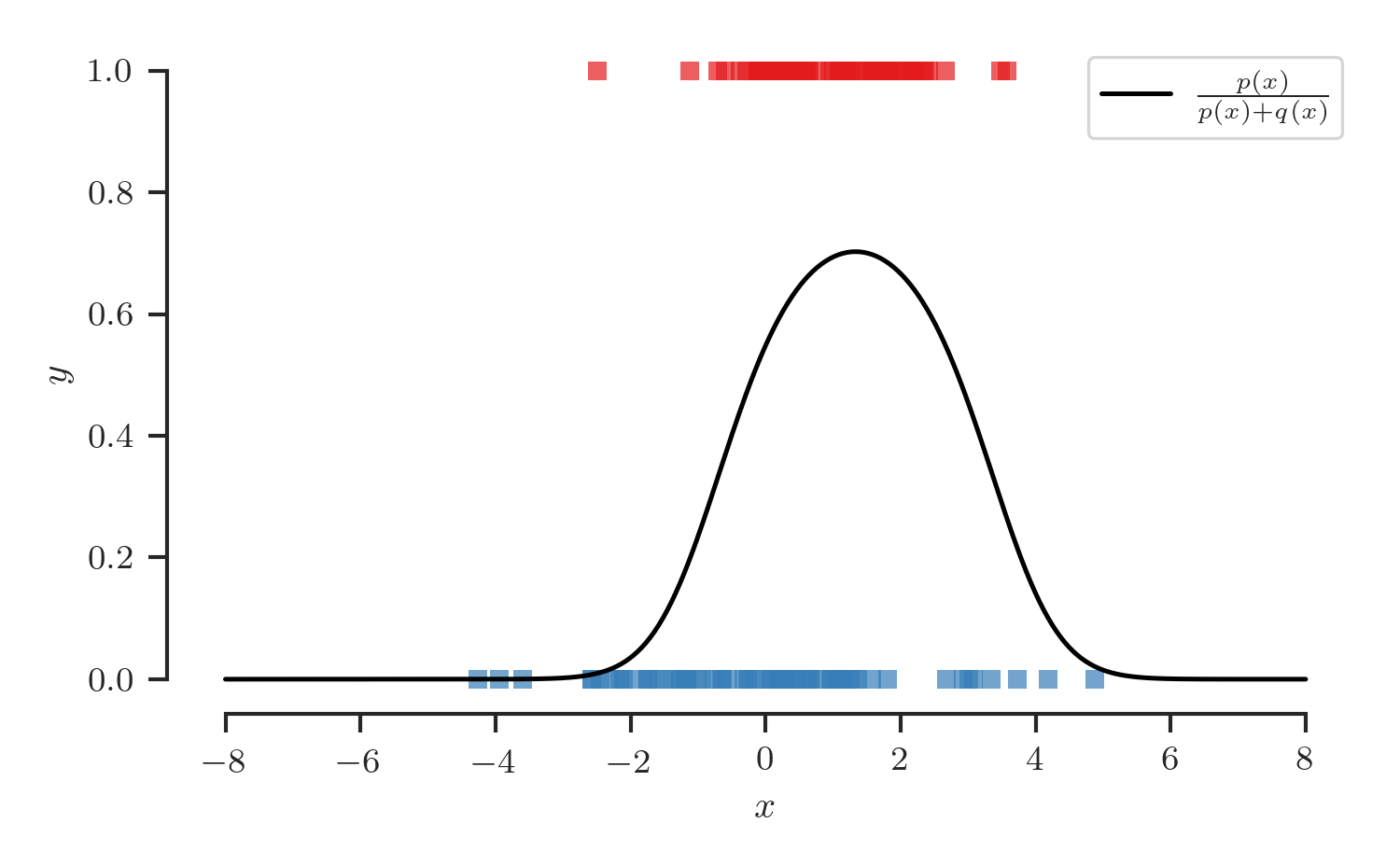
Classification dataset $\mathcal{D}_N = \{(\mathbf{x}_n, y_n)\}_{n=1}^N$ and the true class-posterior probability.
Running CAVI is then a matter of
kappa = y_train - 0.5
Phi = basis_function(X_train, degree=3)

mu, Sigma, xi = cavi(Phi, kappa, alpha=2.0)
The figures below trace the variational parameters over iterations, with hues progressing along a perceptually uniform colormap as in Part II. First, the local parameters $\xi_n$, plotted at their corresponding input locations $x_n$:
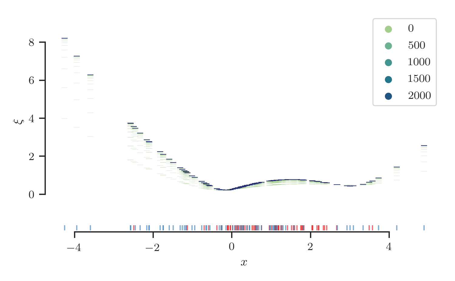
Local variational parameters $\xi_n$ over CAVI iterations, placed at their input locations $x_n$. Since $\xi_n^2 = \mathbb{E}[\psi_n^2]$, the converged values track the (root-mean-square) magnitude of the latent function at each input.
The corresponding expectations $\lambda(\xi_n) = \mathbb{E}_q[\omega_n]$, which play the role Part II’s sampled $\omega_n$ played:
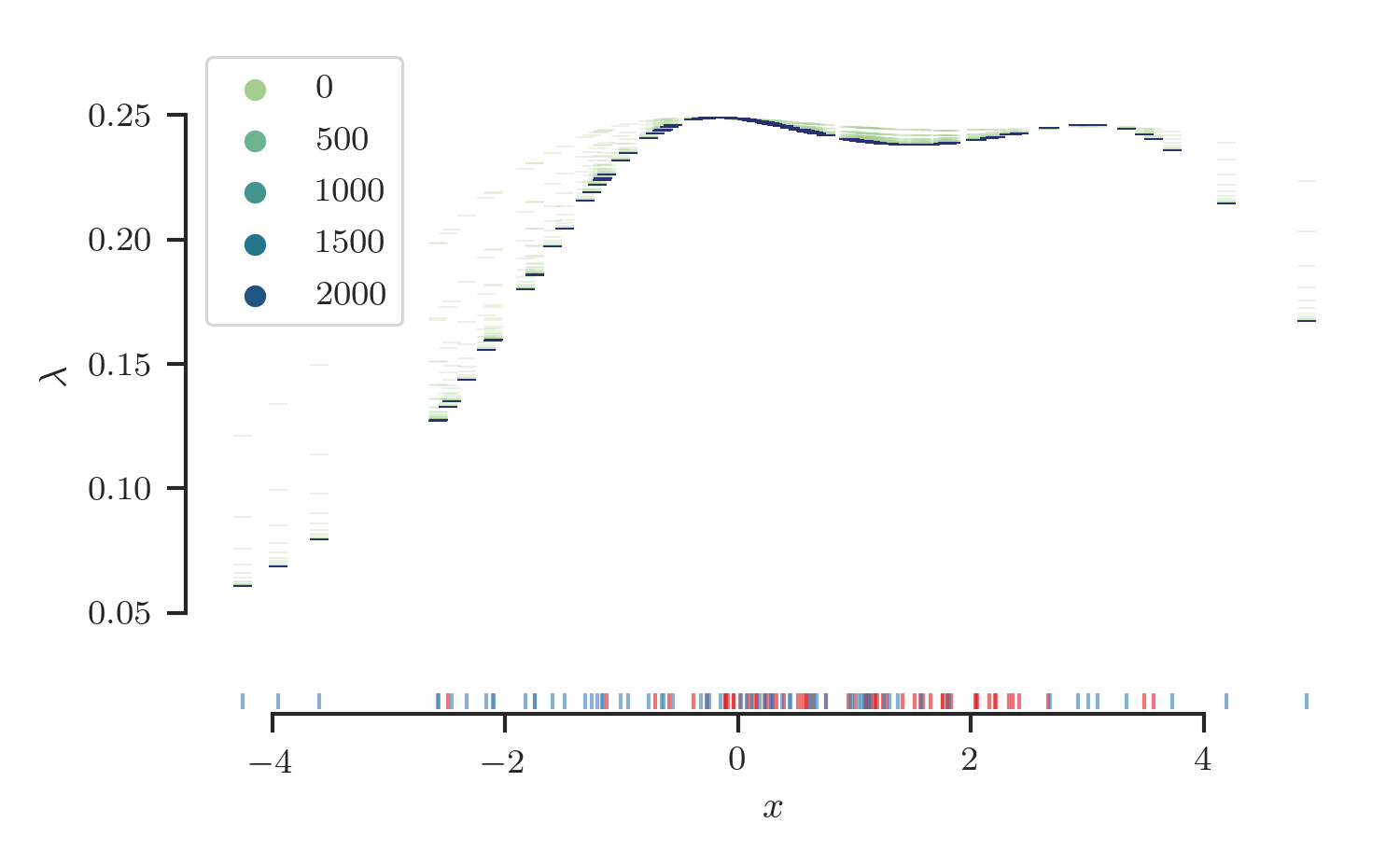
Variational means $\lambda(\xi_n) = \mathbb{E}_{q}[\omega_n]$ over CAVI iterations. Compare with the sampled $\omega_n$ in Part II: large where the classifier is uncertain, small where $|\psi_n|$ is large.
The trajectory of the variational mean $\boldsymbol{\mu}$, which (unlike its Gibbs counterpart) converges to a point:
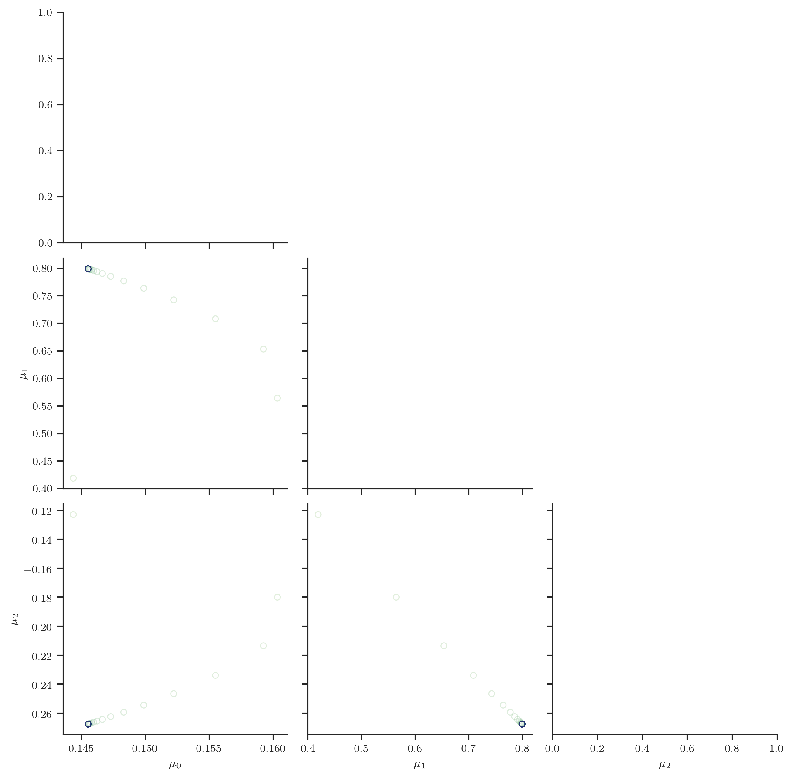
Trajectory of the variational mean $\boldsymbol{\mu}$ across CAVI iterations, shown pairwise for the three basis coefficients. The iterates march deterministically to a fixed point rather than bouncing around a posterior.
And the induced class-membership probability predictions over iterations:
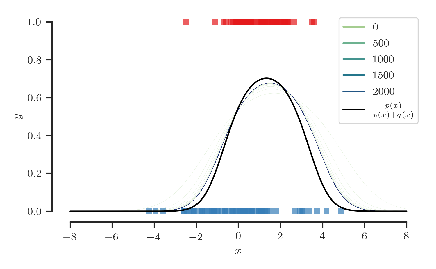
Predicted class-membership probability $\sigma(\phi(x)^{\top} \boldsymbol{\mu})$ as CAVI iterations progress.
Convergence takes a few dozen iterations, each costing one solve of a $K \times K$ linear system. There is no burn-in to diagnose and no seed to worry about; running it twice gives the same answer to machine precision.
Gibbs versus CAVI
Since Parts II and III solve the same problem on the same data (same seed,
even), we owe ourselves the comparison. The script compare.py in this
post’s source bundle runs both algorithms side by side: 5,000 Gibbs sweeps
(1,000 discarded as burn-in) against CAVI run to convergence.
The posterior means agree to about a percent: $\boldsymbol{\mu}_{\text{Gibbs}} = (0.144, 0.809, -0.272)$ versus $\boldsymbol{\mu}_{\text{CAVI}} = (0.146, 0.799, -0.267)$. The posterior spreads do not: coordinate-wise, the variational standard deviations are $0.95\times$, $0.68\times$ and $0.70\times$ their Gibbs counterparts.
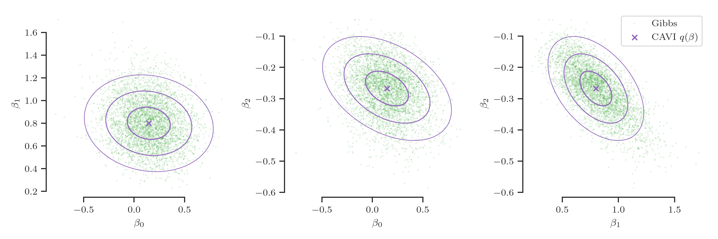
Posterior over the weights $\boldsymbol{\beta}$, pairwise: Gibbs samples (green) against the Gaussian $q(\boldsymbol{\beta})$ (purple; 1, 2 and 3 standard-deviation contours). The orientation is right and the location is right; the volume is not.
This is the textbook mean-field failure mode, and the structural remark from earlier tells us exactly whom to blame. The ellipses are correctly oriented because $q(\boldsymbol{\beta})$ carries a full covariance matrix; correlations between weights are represented. What the factorization discards is the coupling between $\boldsymbol{\beta}$ and $\boldsymbol{\omega}$: the exact posterior accounts for uncertainty in the $\omega_n$ when spreading out $\boldsymbol{\beta}$, whereas the variational posterior conditions on their fixed expectations $\lambda(\xi_n)$, and is overconfident accordingly.
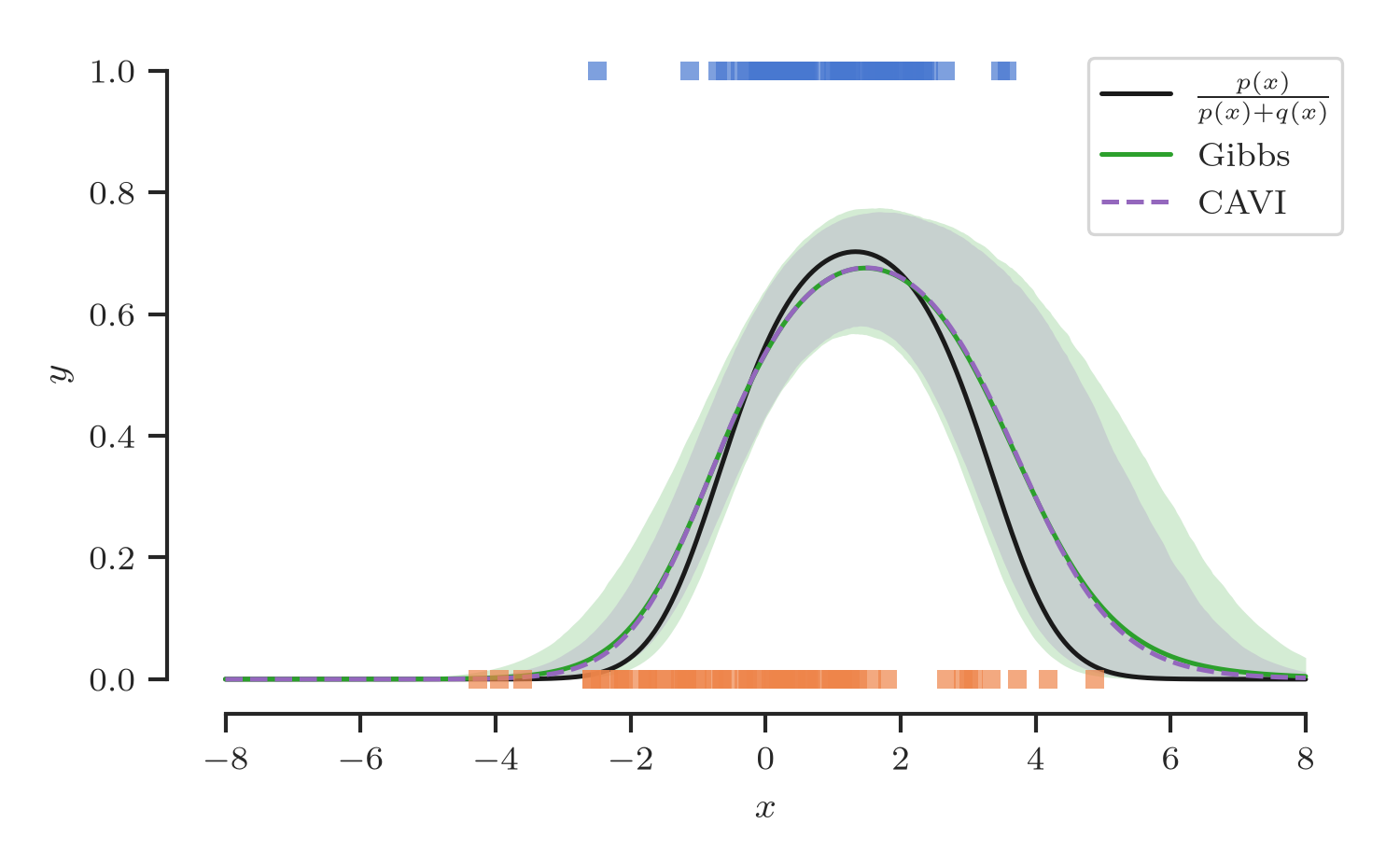
Posterior predictive class probability: Gibbs (green, with 95% band) against CAVI (purple, dashed, with 95% band), and the true class probability (black). The predictive means are visually indistinguishable; the variational band is visibly narrower, most noticeably where the model extrapolates.
On predictions the story is the same in miniature. The two predictive means essentially coincide, and both track the truth about as well as a degree-3 polynomial classifier fit to 128 points has any right to. The variational credible band is narrower everywhere, most visibly in the extrapolation regions beyond the data, where the Gibbs posterior is honest about its ignorance and the mean-field posterior is not.
Whether this trade is acceptable is problem-dependent. CAVI converged in a few dozen deterministic iterations; Gibbs needed thousands of sweeps, each requiring $N$ Pólya-gamma draws. On this toy problem both run in the blink of an eye, and the case for VI is aesthetic at best. The case becomes practical when $N$ grows (the ELBO admits stochastic optimization over mini-batches) or when the model is embedded in a larger system that needs gradients and determinism rather than samples.
The Classical Route
None of the machinery above existed when the bound was first derived. The Pólya-gamma distribution entered the literature with Polson et al. in 20135; Jaakkola and Jordan published in 2000, with workshop versions circulating since the mid-1990s. Their route was convex analysis, and it is worth walking briefly, both for history and because it is genuinely slick.
Start from the decomposition $\log{\sigma(\psi)} = \frac{\psi}{2} - \log{\left(2\cosh{\left(\frac{\psi}{2}\right)}\right)}$ and regard the awkward second term as a function of $t = \psi^2$:
$$ f(t) \triangleq -\log{\left(2\cosh{\left(\frac{\sqrt{t}}{2}\right)}\right)}. $$A short calculation shows $f'(t) = -\frac{\lambda(\sqrt{t})}{2}$, and since $\lambda$ is strictly decreasing on $(0, \infty)$, $f'$ is increasing; $f$ is convex in $t$. A convex function lies above its tangents, so taking the tangent at $t_0 = \xi^2$,
$$ f(t) \geq f(\xi^2) + f'(\xi^2) \, (t - \xi^2) = f(\xi^2) - \frac{\lambda(\xi)}{2} (\psi^2 - \xi^2), $$and adding back $\frac{\psi}{2}$ yields precisely $\log{\sigma(\psi)} \geq \log{\ell(\psi, \xi)}$, with equality where the tangent touches, at $\psi^2 = \xi^2$. The bound is linear in $\psi^2$, which is what makes it exponential-quadratic in $\psi$ and therefore conjugate to a Gaussian prior — the whole point of the exercise.
Equivalently, one can state the result as an upper bound on the softplus function $\varsigma(\psi) \triangleq \log{(1 + e^{\psi})}$, which is how it is often deployed (and how it generalizes to the multi-class case6):
$$ \varsigma(\psi) \leq \frac{\psi - \xi}{2} + \frac{\lambda(\xi)}{2} (\psi^2 - \xi^2) + \varsigma(\xi) \triangleq g(\psi, \xi). $$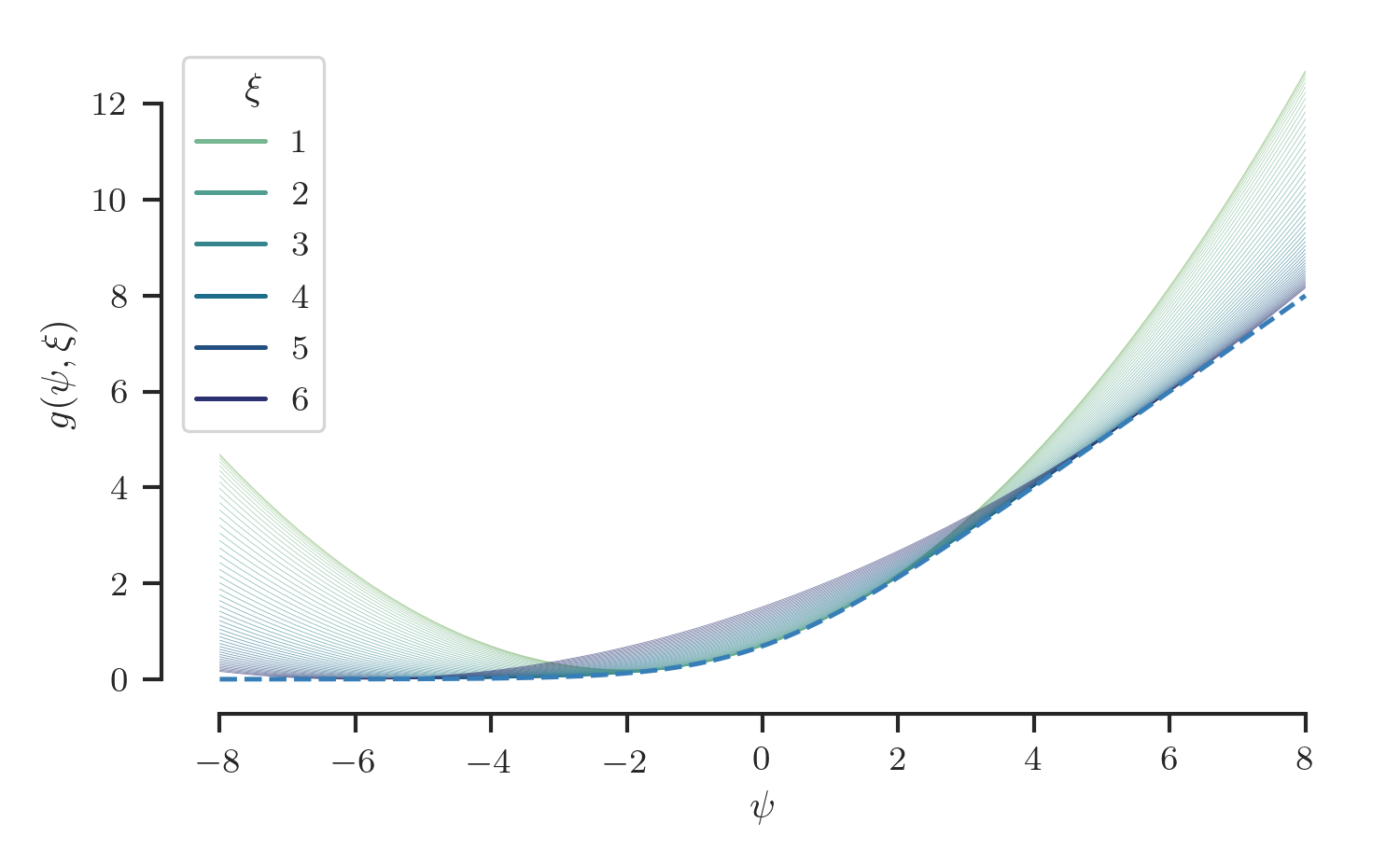
The softplus function (dashed) and the family of quadratic upper bounds $g(\psi, \xi)$, one curve per value of $\xi$.
The two forms are related through $\log{\sigma(\psi)} = -\varsigma(-\psi)$: bounding one from above bounds the other from below,
$$ \begin{align*} \log{\sigma(\psi)} = - \varsigma(- \psi) & \geq -g(-\psi, \xi) \newline & = \frac{\psi + \xi}{2} - \frac{\lambda(\xi)}{2} (\psi^2 - \xi^2) - \varsigma(\xi) \newline & = \frac{\psi - \xi}{2} - \frac{\lambda(\xi)}{2} (\psi^2 - \xi^2) + \log{\sigma(\xi)} \newline & = \log{\ell(\psi, \xi)}, \end{align*} $$where the last step uses $\frac{\xi}{2} - \varsigma(\xi) = -\frac{\xi}{2} - \varsigma(-\xi) = \log{\sigma(\xi)} - \frac{\xi}{2}$, an identity from Part I.
In Jaakkola and Jordan’s paper the coefficient appears as $\lambda_{\text{JJ}}(\xi) = \frac{1}{2\xi}\left(\sigma(\xi) - \frac{1}{2}\right)$, and since $\sigma(\xi) - \frac{1}{2} = \frac{1}{2}\tanh{\left(\frac{\xi}{2}\right)}$, this is $\frac{1}{4\xi}\tanh{\left(\frac{\xi}{2}\right)} = \frac{\lambda(\xi)}{2}$: half the mean of a distribution that would not be described for another decade and a half. From the classical route, $\lambda$ is the derivative of a convex function and its form is a computation. From the variational route, it is the mean of the variational factor over $\omega$. Polson et al. supplied the missing distribution; Durante and Rigon supplied the missing sentence.
Where This Goes
Everything in this post extends along the same lines as the augmentation itself. Likelihoods of the form $\frac{(e^{\psi})^a}{(1 + e^{\psi})^b}$ admit $\mathrm{PG}(b, \cdot)$ auxiliary variables, which covers binomial counts and negative-binomial models. The multi-class softmax has its own quadratic bounds6 and its own augmentation strategies, such as the one-vs-each construction used for Gaussian process classification7. And replacing our fixed-form $q(\boldsymbol{\beta})$ updates with natural-gradient steps on mini-batches gives the scalable Gaussian process classifiers of Wenzel et al.8, which is the modern reason to care about any of this at scale.
The general moral is worth carrying around: when a local variational bound with one parameter per datapoint appears in the literature, it is worth asking which augmented model it is secretly the mean-field ELBO of. For the logistic likelihood the answer took fifteen years to arrive. The next quadratic bound you meet may come with its explanation already attached.
Links and Further Readings
- Papers:
- The local variational method (Jaakkola & Jordan, 2000)1
- The Pólya-gamma augmentation (Polson et al., 2013)5
- The formal equivalence between the two (Durante & Rigon, 2019)3
- Extended to GP classification (Wenzel et al., 2019)8
- Few-shot classification with GPs and the one-vs-each likelihood (Snell et al., 2020)7
- Book chapters:
- Bishop’s PRML, Section 10.6 “Variational Logistic Regression”2
- Blog posts:
- Pólya-Gamma Augmentation by G. Gundersen
- Code:
- The scripts reproducing every figure in this post live in the post’s
source bundle (
src/); the comparison and verification scripts are self-contained and run withuv run.
- The scripts reproducing every figure in this post live in the post’s
source bundle (
Cite as:
@article{tiao2021polyagammalocal,
  title   = "{A} {P}rimer on {P}ólya-gamma {R}andom {V}ariables - {P}art III: {L}ocal {V}ariational {M}ethods",
  author  = "Tiao, Louis C",
  journal = "tiao.io",
  year    = "2021",
  url     = "https://tiao.io/post/polya-gamma-sigmoid-local-variational-lower-bound/"
}
To receive updates on more posts like this, follow me on Twitter and GitHub!
Appendix
I
We derive the closed form of $\mathrm{KL}[\, \mathrm{PG}(1, \xi) \, \| \, \mathrm{PG}(1, \psi) \,]$ and the slack identity. Both distributions are exponential tiltings of the base measure $\mathrm{PG}(\omega | 1, 0)$,
$$ \mathrm{PG}(\omega | 1, c) = \cosh{\left(\frac{c}{2}\right)} \exp{\left(-\frac{c^2}{2}\omega\right)} \mathrm{PG}(\omega | 1, 0), $$so their log-ratio is affine in $\omega$,
$$ \begin{align*} & \log \frac{\mathrm{PG}(\omega | 1, \xi)}{\mathrm{PG}(\omega | 1, \psi)} = \newline & \qquad \log{\cosh{\left(\frac{\xi}{2}\right)}} - \log{\cosh{\left(\frac{\psi}{2}\right)}} + \frac{\psi^2 - \xi^2}{2} \omega. \end{align*} $$Taking the expectation under $\mathrm{PG}(1, \xi)$, whose mean is $\lambda(\xi)$, gives
$$ \begin{align*} & \mathrm{KL}[\, \mathrm{PG}(1, \xi) \, \| \, \mathrm{PG}(1, \psi) \,] = \newline & \qquad \log{\cosh{\left(\frac{\xi}{2}\right)}} - \log{\cosh{\left(\frac{\psi}{2}\right)}} + \frac{\psi^2 - \xi^2}{2} \lambda(\xi). \end{align*} $$For the slack identity, expand $\log{\ell}$:
$$ \begin{align*} & \log{\sigma(\psi)} - \log{\ell(\psi, \xi)} \newline & \quad = \log{\sigma(\psi)} - \log{\sigma(\xi)} - \frac{\psi - \xi}{2} + \frac{\lambda(\xi)}{2}(\psi^2 - \xi^2) \newline & \quad = \log{\cosh{\left(\frac{\xi}{2}\right)}} - \log{\cosh{\left(\frac{\psi}{2}\right)}} + \frac{\psi^2 - \xi^2}{2} \lambda(\xi) \newline & \quad = \mathrm{KL}[\, \mathrm{PG}(1, \xi) \, \| \, \mathrm{PG}(1, \psi) \,], \end{align*} $$where the second equality applies $\log{\sigma(u)} = \frac{u}{2} - \log{\left(2\cosh{\left(\frac{u}{2}\right)}\right)}$ (Part I) to both sigmoid terms: the resulting $\frac{\psi - \xi}{2}$ cancels against the $-\frac{\psi - \xi}{2}$ already present, and the two $\log 2$ constants cancel each other. The same computation with $-\psi$ in place of $\psi$ covers the $y = 0$ case, since the KL divergence depends on $\psi$ only through $\psi^2$; the gap $\log{p(y | \boldsymbol{\beta})} - H(y, \xi, \boldsymbol{\beta})$ is independent of $y$.
Jaakkola, T. S., & Jordan, M. I. (2000). Bayesian Parameter Estimation via Variational Methods. Statistics and Computing, 10(1), 25-37. ↩︎ ↩︎
Bishop, C. M. (2006). Pattern Recognition and Machine Learning. Springer. Section 10.6. ↩︎ ↩︎
Durante, D., & Rigon, T. (2019). Conditionally Conjugate Mean-Field Variational Bayes for Logistic Models. Statistical Science, 34(3), 472-485. ↩︎ ↩︎ ↩︎
A convention warning for readers cross-referencing the original papers: Jaakkola and Jordan (and, following them, Bishop) define $\lambda_{\text{JJ}}(\xi) = \frac{1}{4\xi}\tanh{\left(\frac{\xi}{2}\right)}$, which is half of our $\lambda(\xi)$. Their exponent carries $\lambda_{\text{JJ}}(\xi)(\psi^2 - \xi^2)$ where ours carries $\frac{\lambda(\xi)}{2}(\psi^2 - \xi^2)$; the bounds are identical. We prefer this normalization because it makes $\lambda(\xi)$ exactly the Pólya-gamma mean $\mathbb{E}_{\mathrm{PG}(1,\xi)}[\omega]$. ↩︎
Polson, N. G., Scott, J. G., & Windle, J. (2013). Bayesian Inference for Logistic Models using Pólya–Gamma Latent Variables. Journal of the American Statistical Association, 108(504), 1339-1349. ↩︎ ↩︎
Bouchard, G. (2007). Efficient Bounds for the Softmax Function, Applications to Inference in Hybrid Models. In Presentation at the Workshop for Approximate Bayesian Inference in Continuous/Hybrid Systems at NIPS2007. ↩︎ ↩︎
Snell, J., & Zemel, R. (2020). Bayesian Few-Shot Classification with One-vs-Each Pólya-Gamma Augmented Gaussian Processes. arXiv preprint arXiv:2007.10417. ↩︎ ↩︎
Wenzel, F., Galy-Fajou, T., Donner, C., Kloft, M., & Opper, M. (2019, July). Efficient Gaussian Process Classification using Pòlya-Gamma Data Augmentation. In Proceedings of the AAAI Conference on Artificial Intelligence (Vol. 33, No. 01, pp. 5417-5424). ↩︎ ↩︎
