A Primer on Pólya-gamma Random Variables - Part I: Basic Relationships

This is Part I of a three-part series on Pólya-Gamma random variables. See also: Part II — Bayesian Logistic Regression and Part III — Local Variational Methods.
Table of Contents
A recurring nuisance in Bayesian statistics is that the likelihoods we want and the priors we can compute with refuse to cooperate. Bayesian logistic regression is the canonical example: the Bernoulli likelihood with a logit link is not conjugate to a Gaussian prior, the posterior has no closed form, and one ordinarily reaches for approximations (the Laplace approximation, variational inference, expectation propagation) or for sampling (MCMC). We have collectively made peace with this state of affairs, to the point where it is easy to forget there is anything to make peace with.
The Pólya-gamma augmentation of Polson, Scott, and Windle1 offers a different bargain: introduce auxiliary random variables, chosen so that the awkward likelihood becomes conditionally Gaussian, and the non-conjugate model becomes conjugate again, conditioned on the right things. No approximation is involved; the augmented model is the original model, exactly.
This series builds the trick up from its parts. In this first post we lay out the small collection of identities that make everything work, relating the logistic sigmoid to the hyperbolic cosine, and the hyperbolic cosine to the Laplace transform of the Pólya-gamma distribution. There are no models and no data here; just the moving parts, each verified numerically before we trust it with anything. Part II assembles these parts into Bayesian logistic regression with an exact Gibbs sampler, and Part III swaps the sampler for variational inference and finds a classical method hiding inside.
The Sigmoid, via the Hyperbolic Cosine
Our protagonist is the ubiquitous logistic sigmoid function,
$$ \sigma(u) = \frac{1}{1 + \exp{(-u)}}, $$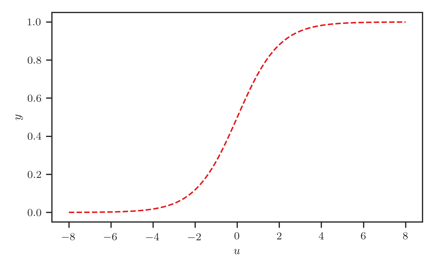
The logistic sigmoid function.
and our first supporting character is the hyperbolic cosine,
$$ \cosh(u) = \frac{e^{u} + e^{-u}}{2}. $$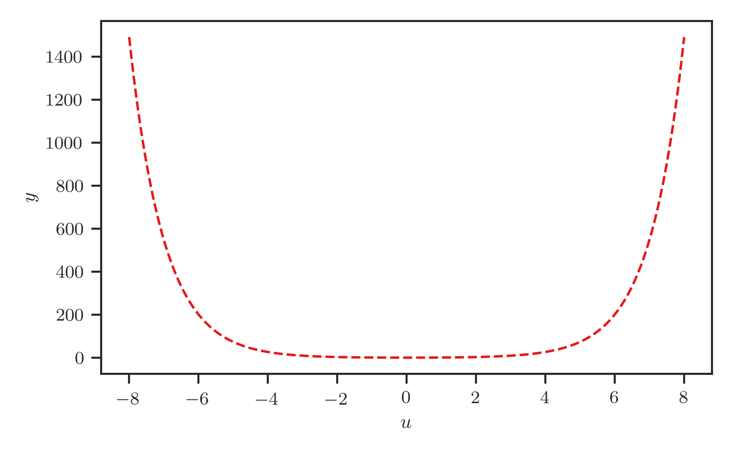
The hyperbolic cosine function.
Identity 1
The two are related by
$$ \sigma(u) = \frac{e^{\frac{u}{2}}}{2\cosh(\frac{u}{2})}. $$This might be immediately obvious for some, but it wasn’t for me. Here is the approach I took to derive it. First, note that
$$ \frac{1}{2\cosh(\frac{u}{2})} = \frac{1}{e^{\frac{u}{2}} + e^{-\frac{u}{2}}}. $$Multiplying by $1 = \frac{e^{\frac{u}{2}}}{e^{\frac{u}{2}}}$ gives
$$ \sigma(u) = \frac{e^{\frac{u}{2}}}{e^{\frac{u}{2}}} \frac{1}{1 + e^{-u}} = \frac{e^{\frac{u}{2}}}{e^{\frac{u}{2}} + e^{-\frac{u}{2}}} = \frac{e^{\frac{u}{2}}}{2\cosh(\frac{u}{2})}. $$Taking logarithms yields a form that Parts II and III will lean on repeatedly:
$$ \log{\sigma(u)} = \frac{u}{2} - \log{\left(2\cosh{\left(\frac{u}{2}\right)}\right)}. $$The point of the maneuver is that the denominator $2\cosh(\frac{u}{2})$, unlike $1 + e^{-u}$, is something we are about to express as an expectation.
The Pólya-Gamma Distribution
Enter the second supporting character.
Pólya-gamma distribution (Polson et al. 2013)
A random variable $\omega$ has a Pólya-gamma distribution with parameters $b > 0$ and $c \in \mathbb{R}$, denoted $\omega \sim \mathrm{PG}(b, c)$, if
$$ \omega \overset{D}{=} \frac{1}{2 \pi^2} \sum_{k=1}^{\infty} \frac{g_k}{\left (k - \frac{1}{2} \right )^2 + \left ( \frac{c}{2\pi} \right )^2} $$where the $g_k \sim \mathrm{Ga}(b, 1)$ are independent gamma random variables (and where $\overset{D}{=}$ denotes equality in distribution).
The distribution is supported on the positive reals; $b$ acts as a shape parameter and $c$ as a tilting parameter (more on the latter in Part II). The infinite sum means the density has no closed form, which sounds disqualifying for a distribution we intend to build models out of. The saving grace, and the reason the distribution was constructed this way in the first place, is that its Laplace transform has a very pleasant closed form indeed.
Sampling is a solved problem: Polson and Windle devised efficient exact samplers2, available in Python via the polyagamma package,
import numpy as np
from polyagamma import random_polyagamma

rng = np.random.default_rng(8888)
omega = random_polyagamma(1, 0, size=32, random_state=rng)
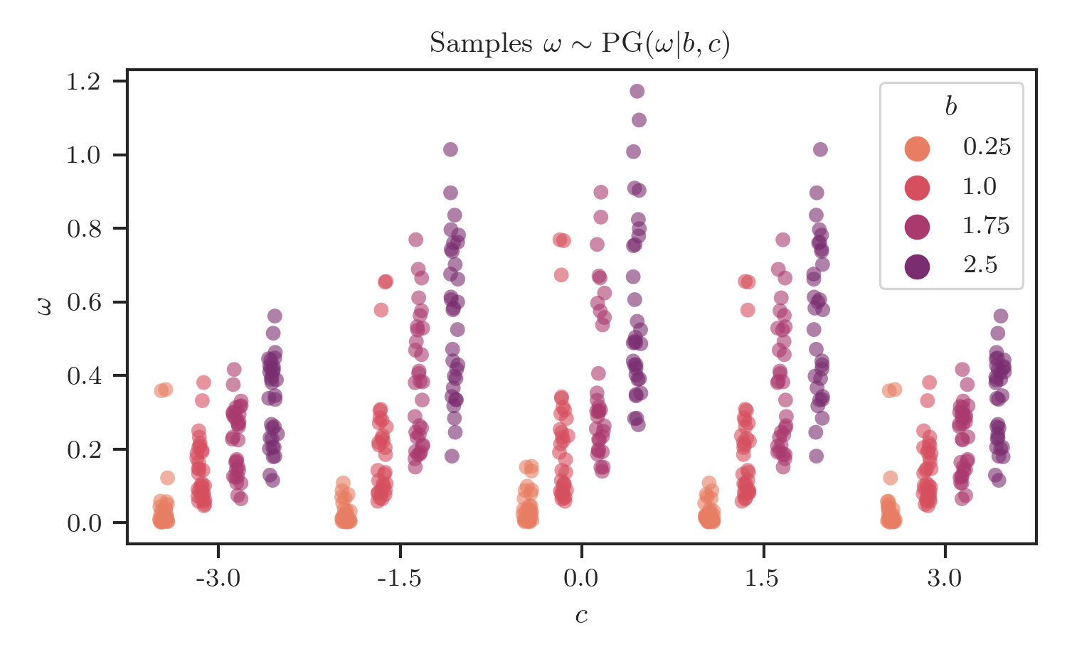
Samples $\omega \sim \mathrm{PG}(b, c)$ across a range of tilting parameters $c$, colored by shape parameter $b$ (32 draws per configuration).
The Laplace Transform
Laplace transform of the Pólya-gamma distribution (Polson et al. 2013)
For $\omega \sim \mathrm{PG}(b, 0)$,
$$ \mathbb{E}_{\mathrm{PG}(\omega | b, 0)}[\exp{(- \omega t)}] = \frac{1}{\cosh^b{\left (\sqrt {\frac{t}{2}} \right )}}. $$Identity 2
There is a hyperbolic cosine, conveniently in a denominator. To make it match the one in Identity 1, set $b=1$ and reparameterize
$$ t = \frac{u^2}{2} \Leftrightarrow \frac{t}{2} = \left ( \frac{u}{2} \right )^2 \Leftrightarrow \sqrt{\frac{t}{2}} = \frac{u}{2}, $$which gives
$$ \mathbb{E}_{\mathrm{PG}(\omega | 1, 0)} \left [\exp{ \left (- \frac{u^2}{2} \omega \right )} \right ] = \frac{1}{\cosh{\left ( \frac{u}{2} \right )}}. $$Combining with Identity 1, the sigmoid becomes an expectation with respect to a Pólya-gamma random variable:
$$ \sigma(u) = \frac{e^{\frac{u}{2}}}{2 \cosh{\left ( \frac{u}{2} \right )}} = \frac{1}{2} \mathbb{E}_{\mathrm{PG}(\omega | 1, 0)} \left [\exp{ \left (\frac{u}{2} - \frac{u^2}{2} \omega \right )} \right ]. $$This is the identity the entire series stands on. Everything in Parts II and III is a consequence of the fact that the exponent on the right-hand side is quadratic in $u$.
A Mixture of Gaussian Kernels
To see the quadratic structure clearly, give the integrand a name,
$$ k(u, \omega) \triangleq \frac{1}{2} \exp{ \left (\frac{u}{2} - \frac{u^2}{2} \omega \right )}, $$so that
$$ \sigma(u) = \int k(u, \omega) \, \mathrm{PG}(\omega | 1, 0) \, \mathrm{d}\omega. $$It is tempting to read this as a joint density $p(u, \omega)$ with conditional $k$ and marginal $\sigma$. Resist the temptation: $\sigma$ is not integrable in $u$ (it tends to $1$ as $u \to \infty$), and $k(\cdot, \omega)$ is not a normalized density either. What we have is an integral representation of the function $\sigma$ rather than a probability model. The genuinely probabilistic version arrives in Part II, where the observed random variable is the discrete label $y$ and everything normalizes as it should.
Completing the square in the exponent shows that each kernel is a Gaussian bump in $u$, rescaled:
$$ \begin{align*} k(u, \omega) &= \frac{1}{2} \exp{ \left (\frac{u}{2} - \frac{u^2}{2} \omega \right )} \newline &\propto \exp{ \left \{ - \frac{\omega}{2} \left ( u - \frac{\omega^{-1}}{2} \right )^2 \right \} } \newline &\propto \mathcal{N} \left ( u ; \frac{\omega^{-1}}{2}, \omega^{-1} \right ), \end{align*} $$and more precisely3
$$ k(u, \omega) = \sqrt{\frac{\pi \omega^{-1}}{2}} \exp{ \left ( \frac{\omega^{-1}}{2^3} \right ) } \times \mathcal{N} \left ( u ; \frac{\omega^{-1}}{2}, \omega^{-1} \right ). $$A draw of $\omega$ thus selects a Gaussian kernel centered at $\frac{1}{2\omega}$ with variance $\frac{1}{\omega}$: small $\omega$ gives a wide bump far to the right, large $\omega$ a narrow bump near the origin. The sigmoid is what you get by averaging these bumps over the $\mathrm{PG}(1, 0)$ distribution.
In code, the kernel is a one-liner,
def kernel(u, omega):
    return 0.5 * np.exp(-0.5 * u * (u * omega - 1.0))
or, in its rescaled-Gaussian form,
from scipy.stats import norm


def kernel(u, omega):

    var = np.reciprocal(omega)

    loc = 0.5 * var
    scale = np.sqrt(var)

    rv = norm(loc=loc, scale=scale)

    return np.sqrt(0.5 * np.pi) * scale * np.exp(0.5**2 * loc) * rv.pdf(u)
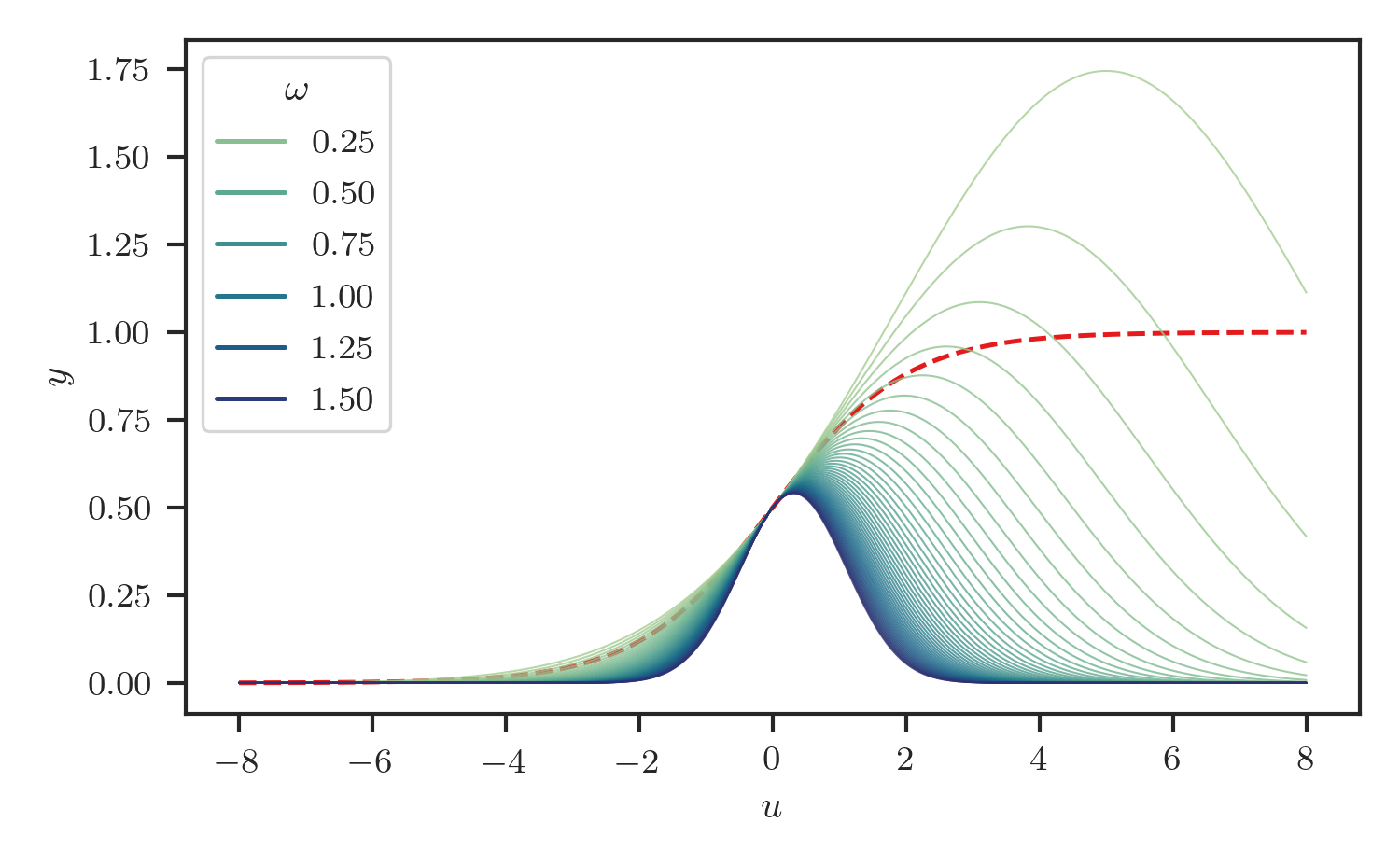
The Gaussian kernels $k(u, \omega)$ as functions of $u$, one curve per value of $\omega$, with the logistic sigmoid $\sigma(u)$ overlaid (dashed). No single kernel resembles the sigmoid; their average will.
Monte Carlo Verification
If the representation is correct, averaging kernels at sampled values of $\omega$ should reproduce the sigmoid:
$$ \begin{align*} \sigma(u) &= \int k(u, \omega) \, \mathrm{PG}(\omega | 1, 0) \, \mathrm{d}\omega \newline &\approx \frac{1}{M} \sum_{m=1}^M k(u, \omega^{(m)}), \qquad \omega^{(m)} \sim \mathrm{PG}(\omega | 1, 0), \end{align*} $$which is two more lines,
omega = random_polyagamma(1, 0, size=1024, random_state=rng)
sigma_hat = kernel(u[:, None], omega).mean(axis=-1)
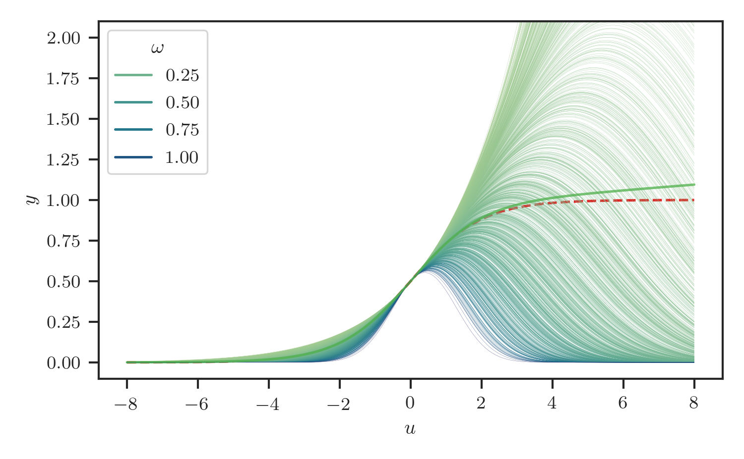
Monte Carlo verification: individual kernels $k(u, \omega^{(m)})$ at prior draws $\omega^{(m)} \sim \mathrm{PG}(1, 0)$, and their running average, which converges to the logistic sigmoid (dashed).
The average hugs the sigmoid, as promised. It is a modest kind of magic: a function famous for ruining conjugacy turns out to be an average of the most conjugacy-friendly objects in existence.
What’s Next
Nothing above involved data, parameters, or a posterior. In Part II we attach this representation to an actual model: the observed variable becomes the binary label $y$, the kernel’s quadratic exponent delivers conditional Gaussian-Gaussian conjugacy, and the resulting conditional posteriors give an exact Gibbs sampler for Bayesian logistic regression. In Part III we run variational inference in the same augmented model and watch the classical Jaakkola-Jordan bound emerge from the ELBO, together with an explanation of why that bound is tight exactly where it is.
Links and Further Readings
- Papers:
- Blog posts:
- Pólya-Gamma Augmentation by G. Gundersen
- Code:
- polyagamma: the actively maintained Python package used above
- pypolyagamma: S. Linderman’s Cython port of BayesLogit, J. Windle’s original R implementation
Cite as:
@article{tiao2021polyagammabasic,
  title   = "{A} {P}rimer on {P}ólya-gamma {R}andom {V}ariables - {P}art I: {B}asic {R}elationships",
  author  = "Tiao, Louis C",
  journal = "tiao.io",
  year    = "2021",
  url     = "https://tiao.io/post/polya-gamma-basic-relationships/"
}
To receive updates on more posts like this, follow me on Twitter and GitHub!
Polson, N. G., Scott, J. G., & Windle, J. (2013). Bayesian Inference for Logistic Models using Pólya–Gamma Latent Variables. Journal of the American Statistical Association, 108(504), 1339-1349. ↩︎ ↩︎
Windle, J., Polson, N. G., & Scott, J. G. (2014). Sampling Pólya-gamma Random Variates: Alternate and Approximate Techniques. arXiv preprint arXiv:1405.0506. ↩︎ ↩︎
Completing the square:
$$ \begin{align*} k(u, \omega) &= \frac{1}{2} \exp{ \left (\frac{u}{2} - \frac{u^2}{2} \omega \right )} \newline &= \frac{1}{2} \exp{ \left \{ - \frac{\omega}{2} \left ( u^2 - u \omega^{-1} \right ) \right \} } \newline &= \frac{1}{2} \exp{ \left \{ \frac{\omega}{2} \left ( \frac{\omega^{-1}}{2} \right )^2 - \frac{\omega}{2} \left ( u - \frac{\omega^{-1}}{2} \right )^2 \right \} } \newline &= \frac{1}{2} \exp{ \left ( \frac{\omega^{-1}}{2^3} \right ) } \times \exp{ \left \{ - \frac{\omega}{2} \left ( u - \frac{\omega^{-1}}{2} \right )^2 \right \} } \newline &= \frac{1}{2} \exp{ \left ( \frac{\omega^{-1}}{2^3} \right ) } \times \frac{\sqrt{2\pi\omega^{-1}}}{\sqrt{2\pi\omega^{-1}}} \exp{ \left \{ - \frac{\omega}{2} \left ( u - \frac{\omega^{-1}}{2} \right )^2 \right \} } \newline &= \sqrt{\frac{\pi \omega^{-1}}{2}} \exp{ \left ( \frac{\omega^{-1}}{2^3} \right ) } \times \mathcal{N} \left ( u ; \frac{\omega^{-1}}{2}, \omega^{-1} \right ) \end{align*} $$ ↩︎
