The Upper Confidence Bound in Disguise

Probability of improvement fixes a threshold $\tau$ and reads off a probability: how much of the predictive mass sits above $\tau$? Expected improvement integrates the gap above $\tau$. The upper confidence bound1 fixes a probability $q$ and reads off a threshold: the value that only $1 - q$ of the mass exceeds. All three are views of the same conditional CDF.
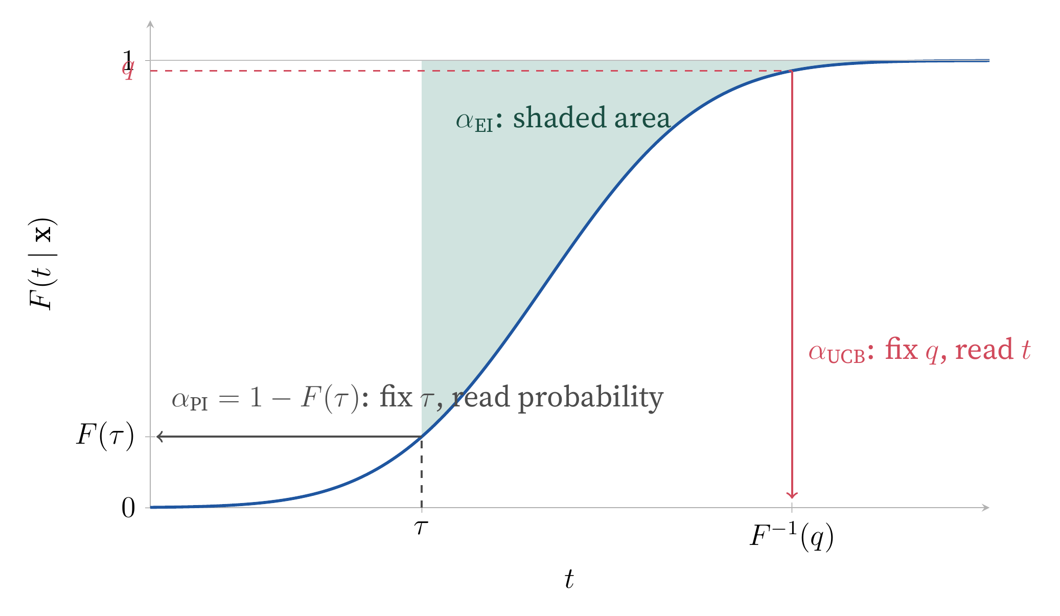
Three views of one conditional CDF. Fix a threshold τ and read off a probability (PI); integrate the gap above the CDF beyond τ (EI); fix a probability q and read off a threshold (UCB).
The third is a quantile. Under a Gaussian predictive, the $q$-quantile is $\mu + \sigma\Phi^{-1}(q)$, which is the UCB formula at $q = \Phi(\sqrt{\beta})$. That matters because quantiles, unlike the moment formula $\mu + \sqrt{\beta}\,\sigma$, come with their own loss function.
Acquisition functions as loss functions
There is a family of methods that replaces the usual surrogate-then-integrate pipeline with supervised learning on raw observations. BORE2 trains a probabilistic classifier on the observed $(\mathbf{x}_i, y_i)$ pairs; after a monotone transform, the classifier’s output is the acquisition function. LFBO3 generalized this into a recipe (the derivation is in the appendix): for any expected utility, there is a classification loss whose empirical minimizer converges to the acquisition function, without ever modeling the predictive distribution. The indicator utility gives PI, the hinge gives EI, and any classifier architecture can stand in for the Gaussian process.
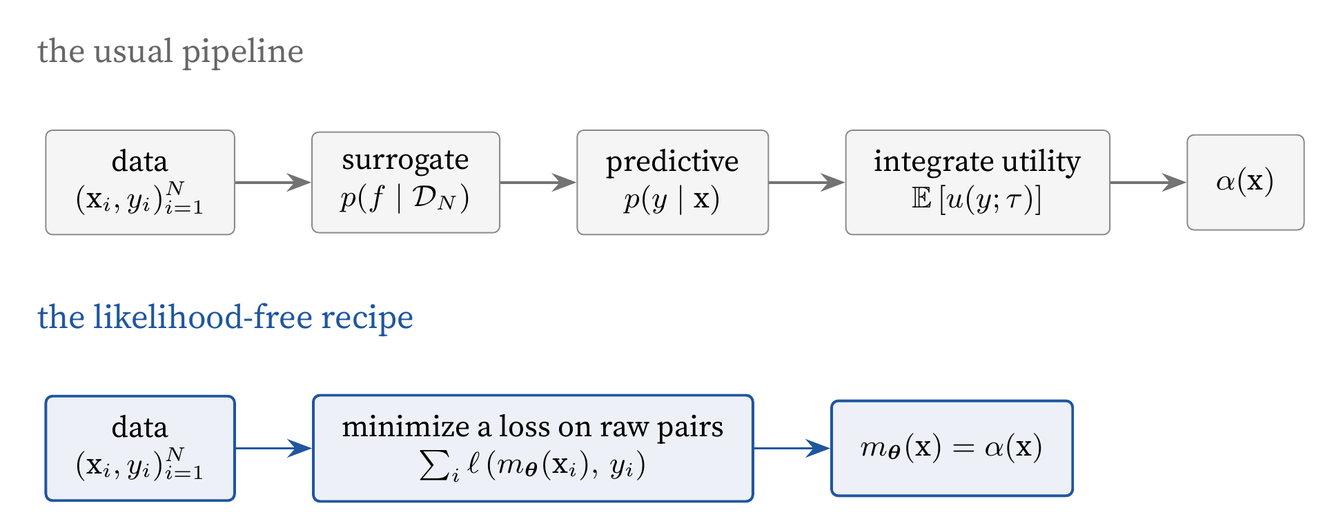
Two routes to an acquisition function. The usual pipeline models the function, forms its predictive, and integrates a utility; the likelihood-free recipe trains on raw pairs, and the trained model is the acquisition function.
PI and EI are where the recipe ends. UCB appears nowhere in this family, and the omission is structural. The recipe can reach some forms of optimism (the entropic risk measure $\mu + \tfrac{k}{2}\sigma^2$ is inside it; see the appendix), but not the scale-equivariant kind that UCB promises.
Conformal quantile regression for hyperparameter optimization,4 from several of my BORE co-authors, took the next step in this lineage. It replaces the classifier with quantile regressors fitted at multiple levels, and selects candidates by independent Thompson sampling: for each candidate, draw one of its predicted quantiles at random and keep the best draw. Its limitations section lists UCB as future work. The extension, it turns out, is the algorithm they already run.
An expectation, but not an expected utility
There is a door that looks open. Wilson et al.5 showed that UCB can be written as an expectation,
$$ \alpha_{\text{UCB}}(\mathbf{x}) = \mathbb{E}_{\gamma}\left[\mu(\mathbf{x}) + |\gamma|\right], \qquad \gamma \sim \mathcal{N}\left(0, \tfrac{\beta\pi}{2}\sigma^2(\mathbf{x})\right), $$since $\mathbb{E}|\gamma| = \sqrt{\beta}\,\sigma$ when the variance is inflated by $\beta\pi/2$. But neither ingredient conforms to the recipe. The integrand contains $\mu(\mathbf{x})$, a functional of the predictive distribution the recipe avoids modeling. And the expectation runs over a variance-inflated law (variance scaled by $\beta\pi/2$ relative to the true predictive) rather than over $p(y \mid \mathbf{x})$; using real observations in its place would require knowing $\mu(\mathbf{x})$ and $\sigma(\mathbf{x})$. The recipe needs a fixed utility and samples from the true conditional. This form supplies neither.
No loss works
What would have to exist is a loss $\ell(z, y)$ whose minimizer over $p$ equals $\mu + \sqrt{\beta}\,\sigma$ for every distribution in the family. The forecasting literature calls a functional with this property elicitable:6 the mean is elicitable (squared loss), the median is elicitable (absolute loss), and quantiles are elicitable. Elicitability is exactly the license a likelihood-free acquisition function needs.
There is a necessary condition, due to Osband: an elicitable functional has convex level sets in distribution space. If two distributions share a value, every mixture of them must share it too. UCB fails this test. In the $(\sigma, \mu)$ half-plane, its level sets are parallel lines of slope $-\sqrt{\beta}$. Means mix linearly, but variances pick up a spread term,
$$ \operatorname{Var}(p_\lambda) = \lambda\sigma_1^2 + (1-\lambda)\sigma_2^2 + \lambda(1-\lambda)(\mu_1 - \mu_2)^2, $$so two distributions on the same level set with different means mix to one that exits upward. $\mathcal{N}(0, 4)$ and $\mathcal{N}(2, 1)$ both have $\mu + 2\sigma = 4$; their even mixture has mean $1$ and $\sigma \approx 1.87$, giving $\mu + 2\sigma \approx 4.74$.
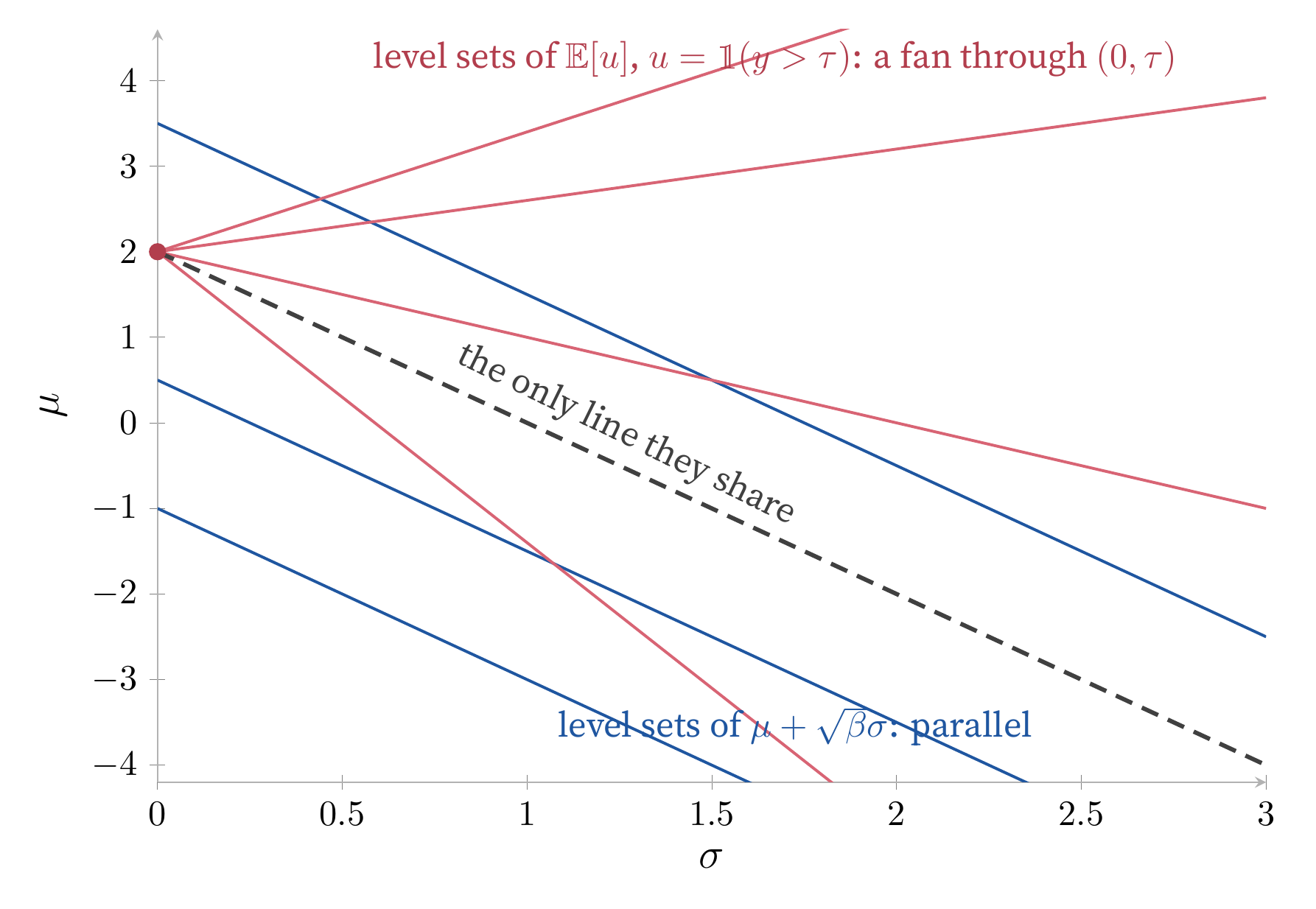
Level sets in the (σ, μ) half-plane. A threshold utility’s expectation fans from (0, τ); UCB’s level sets are parallel lines of slope −√β. A fan and a family of parallels agree on at most one line.
No scalar loss elicits $\mu + \sqrt{\beta}\,\sigma$ over any family closed under mixtures that contains the Gaussians. (An alternative proof via the heat equation appears in the appendix.)
Quantiles come with their own loss
The impossibility condemns the moment formula $\mu + \sqrt{\beta}\,\sigma$. But the opening said UCB is also a quantile, and quantiles are elicitable. The loss that does it is the pinball loss from quantile regression.
Start with what the median does. The median minimizes expected absolute error: overshooting by one unit costs the same as undershooting by one unit, so the optimal prediction sits where the distribution splits evenly. Now tilt the penalty: charge $q$ per unit for undershooting and $1 - q$ per unit for overshooting, and the optimal prediction shifts to the point where a fraction $q$ of the mass lies below. That point is the $q$-quantile. The loss is
$$ \rho_q(r) \triangleq q \max(r, 0) + (1 - q) \max(-r, 0), \qquad r \triangleq y - z, $$and the verification is one line: $\frac{\partial}{\partial z} \mathbb{E}\left[\rho_q(y - z)\right] = F(z) - q$, which vanishes at $z = F^{-1}(q)$.
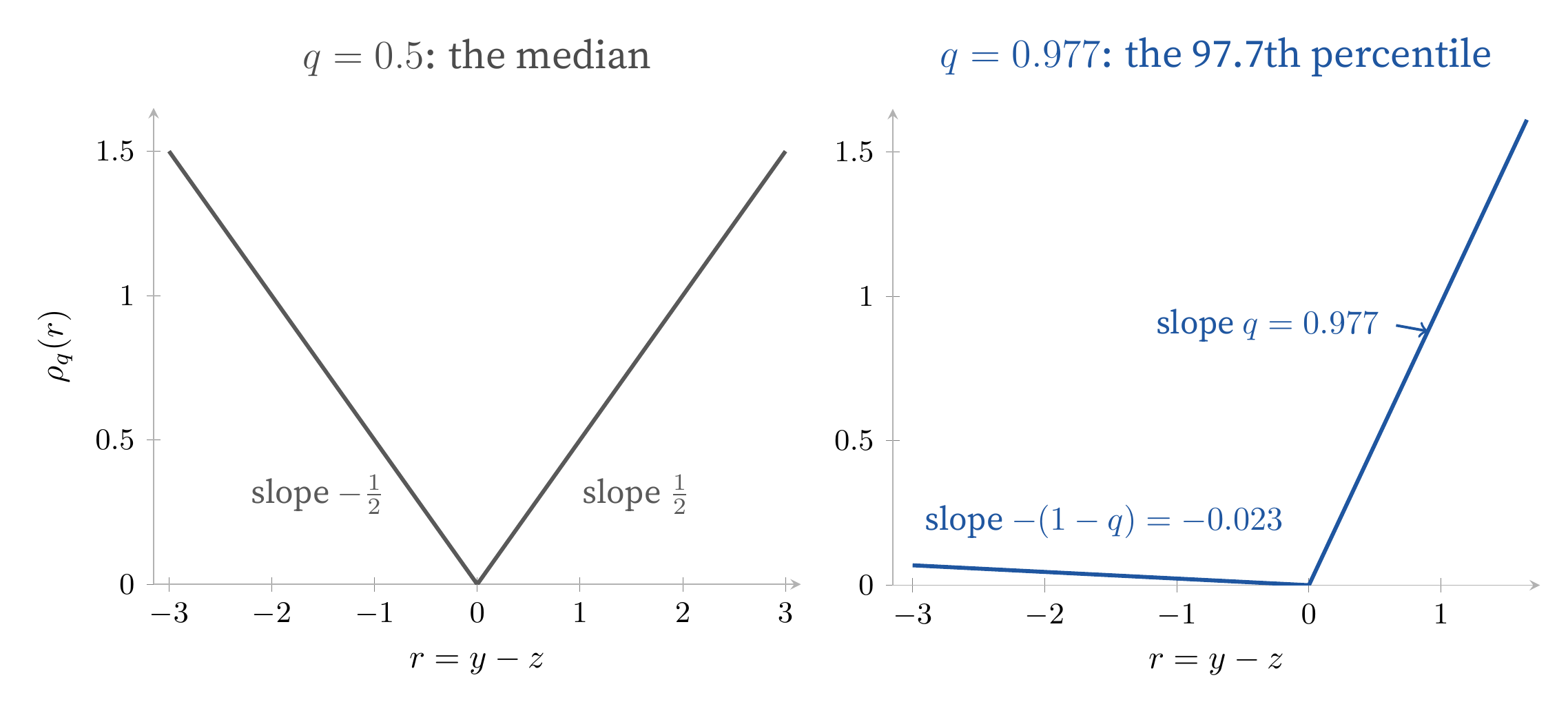
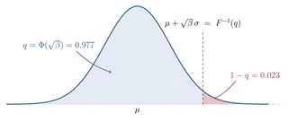
Tilting the median. At q = 0.5 the loss is symmetric absolute error and the minimizer is the median; tilt the slopes to q = 0.977 and the minimizer slides to the 97.7th percentile, where underestimates cost 42 times more than overestimates.
At $q = \Phi(\sqrt{\beta}) \approx 0.977$ for $\beta = 4$, underestimates cost roughly 42 times more than overestimates, so the minimizer parks itself at the 97.7th percentile: exactly the UCB level. Fit a regressor $m_{\boldsymbol{\theta}}$ by minimizing $\sum_i \rho_q(y_i - m_{\boldsymbol{\theta}}(\mathbf{x}_i))$ at that level and maximize its output. The output is the acquisition function, in the units of $y$. No threshold to recompute, no labels to flip. BORE’s quantile fraction $\gamma$ and UCB’s exploration parameter $\beta$, two knobs that looked unrelated, collapse into one: the level $q$.
And there is a subtle upgrade in the swap. When the predictive is not Gaussian, $\mu + \sqrt{\beta}\,\sigma$ and the $q$-quantile genuinely differ, and it is the quantile that keeps meaning what UCB was supposed to mean (the 97.7th percentile of what this candidate might return) while the moment formula drifts. The pinball regressor targets the right object regardless of the noise distribution.
The catch
Honesty requires saying which $\sigma$ this recipe buys. The distribution a pinball regressor learns about is $p(y \mid \mathbf{x})$, the data-generating conditional, so its spread is observation noise: aleatoric uncertainty. The $\sigma(\mathbf{x})$ in GP-UCB is posterior uncertainty about the latent function, which grows away from data and shrinks wherever observations accumulate. That epistemic $\sigma$ is what “optimism in the face of uncertainty” refers to, and no amount of quantile regression on raw pairs recovers it.
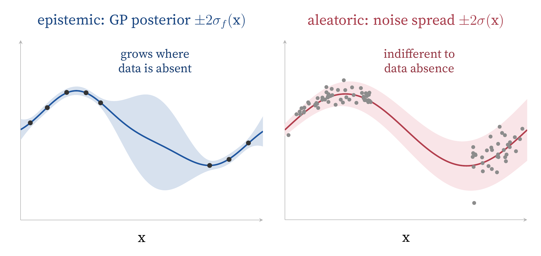
Two σ’s wearing the same letter. The epistemic band of a GP posterior balloons where data is absent; the aleatoric band of the noise itself tracks σ(x) and does not care where you have looked.
On a noiseless objective, $p(y \mid \mathbf{x})$ is a point mass, every quantile equals the objective’s value, and the level $q$ does nothing: the rule degenerates to greedy maximization. Under noise it does something meaningful (it seeks the input whose upper tail is best), but its exploration is optimism about noise rather than optimism about ignorance.
This is not a new debt, and I am poorly placed to complain. BORE and LFBO carry the same one: their classifiers are point estimates, and the exploration they exhibit comes from threshold updates and model misfit rather than from represented uncertainty. But PI and EI never advertised an epistemic term, and UCB is nothing but its epistemic term. (The boundary between what likelihood-free methods can and cannot score is sharper than this; see the appendix.)
The other disguise
Now for the claim from the limitations section. CQR fits $m$ gradient-boosted quantile regressors at equally spaced levels $\alpha_j \triangleq j / (m + 1)$, with $m = 4$ in their experiments, and conformalizes the predictions.7 Its acquisition step is independent Thompson sampling: draw a large pool of candidates, hand each candidate one of its $m$ predicted quantiles uniformly at random as a pseudo-sample, and keep the best draw.
Look at what the sampling step actually computes. The winning draw beats every other draw, including those from candidates whose coin landed on the top level $\alpha_m$ (about a $1/m$ fraction of the pool). Each of those draws is a top-level quantile prediction. Meanwhile the winner’s own top-level quantile can only exceed whatever level it drew, provided the fitted quantiles are monotone across levels. Chain these three facts:
$$ \hat{q}_{\alpha_m}(\mathbf{x}_{\text{sel}}) \geq \text{winning draw} \geq \max_{\mathbf{x} \in \mathcal{D}_{\text{thin}}} \hat{q}_{\alpha_m}(\mathbf{x}). $$Independent Thompson sampling over an $m$-point quantile grid is, at worst, fixed-level quantile maximization over a randomly thinned candidate pool. With their pool of two thousand candidates and $m = 4$, thinning to a quarter changes essentially nothing, and the sampled acquisition collapses onto its deterministic core: maximize $\hat{q}_{\alpha_m}$.
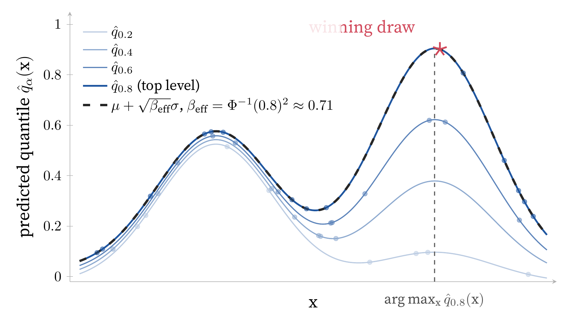
Independent Thompson sampling over four quantile curves: one dot per candidate, placed at its randomly drawn level. The winning draw sits on the top-level curve, at that curve’s maximizer. The black dashes riding the top curve show the analytic UCB at the grid-equivalent level, μ + √β_eff σ with β_eff = Φ⁻¹(0.8)² ≈ 0.71; under this toy’s Gaussian predictive it coincides exactly with the top quantile curve.
With $m = 4$, the top level is $\alpha_4 = 4/5 = 0.8$, and under a Gaussian predictive the 0.8-quantile is $\mu + \Phi^{-1}(0.8)\,\sigma \approx \mu + 0.84\,\sigma$: UCB with $\beta_{\text{eff}} = \Phi^{-1}\!\left(\tfrac{m}{m+1}\right)^{\!2} \approx 0.71$. That is the acquisition function CQR optimizes at its shipped defaults, an exploration bonus of less than one standard deviation. The grid size, chosen as a resolution parameter, has been a $\beta$ dial all along.8
Two honest boundaries: separately fitted quantiles can cross (a possibility their own footnote acknowledges), which adds slack to the monotonicity step in the sandwich; and in sparse pools the thinning genuinely bites, the high-dimensional regime their limitations section already flags.
So the title holds in both directions. UCB is a quantile in disguise, and the leading quantile method is UCB in disguise. Elicitability makes the coincidence unremarkable. Scalar doors to scale-equivariant optimism are scarce (the quantile, and its least-squares cousin the expectile), and on a Gaussian predictive every such functional collapses to $\mu + c\sigma$ for some constant $c$. The limitations section lists UCB as future work. The implementation is already running it.
Appendix
The LFBO derivation
Every differentiable, strictly convex function is the upper envelope of its tangent lines, $f(v) = \max_s \{ v f'(s) - f^{\star}(f'(s)) \}$, where $f^{\star}$ is the convex conjugate. Apply this pointwise to any target function $\alpha$ inside an expectation over candidates, and loosen the pointwise maximization to a single function $S$:
$$ \mathbb{E}_{p(\mathbf{x})}\left[ f(\alpha(\mathbf{x})) \right] \geq \max_{S : \mathcal{X} \to (0, \infty)} \mathbb{E}_{p(\mathbf{x})}\left[ \alpha(\mathbf{x}) f'(S(\mathbf{x})) - f^{\star}\left( f'(S(\mathbf{x})) \right) \right], $$with equality at $S^{\ast} = \alpha$. Take the target to be the expected utility $\alpha_u(\mathbf{x}) \triangleq \mathbb{E}_{p(y \mid \mathbf{x})}[u(y; \tau)]$ for a nonnegative utility $u$ and threshold $\tau$. Since $f'(S(\mathbf{x}))$ does not depend on $y$, the tower rule merges the conditional expectation into the outer one, $\mathbb{E}_{p(\mathbf{x})}[\alpha_u(\mathbf{x}) f'(S(\mathbf{x}))] = \mathbb{E}_{p(\mathbf{x}, y)}[u(y; \tau) f'(S(\mathbf{x}))]$, and the intractable predictive integral dissolves into an average over the raw pairs. Choosing the logistic $f(v) \triangleq v \log v - (v + 1) \log(v + 1)$ and reparameterizing $S = \pi / (1 - \pi)$ lands the objective on weighted binary cross-entropy,
$$ \max_{\pi}\ \mathbb{E}_{p(\mathbf{x}, y)}\left[ u(y; \tau) \log \pi(\mathbf{x}) + \log\left( 1 - \pi(\mathbf{x}) \right) \right], $$in which every observation participates as a negative with weight one and as a positive with weight $u(y_i; \tau)$.9 The logistic choice is arbitrary: any strictly convex $f$ elicits the same $\alpha_u$ at the population optimum, so the choice of divergence changes the training objective but never the functional it recovers. No choice of $f$ reaches beyond expected utilities.
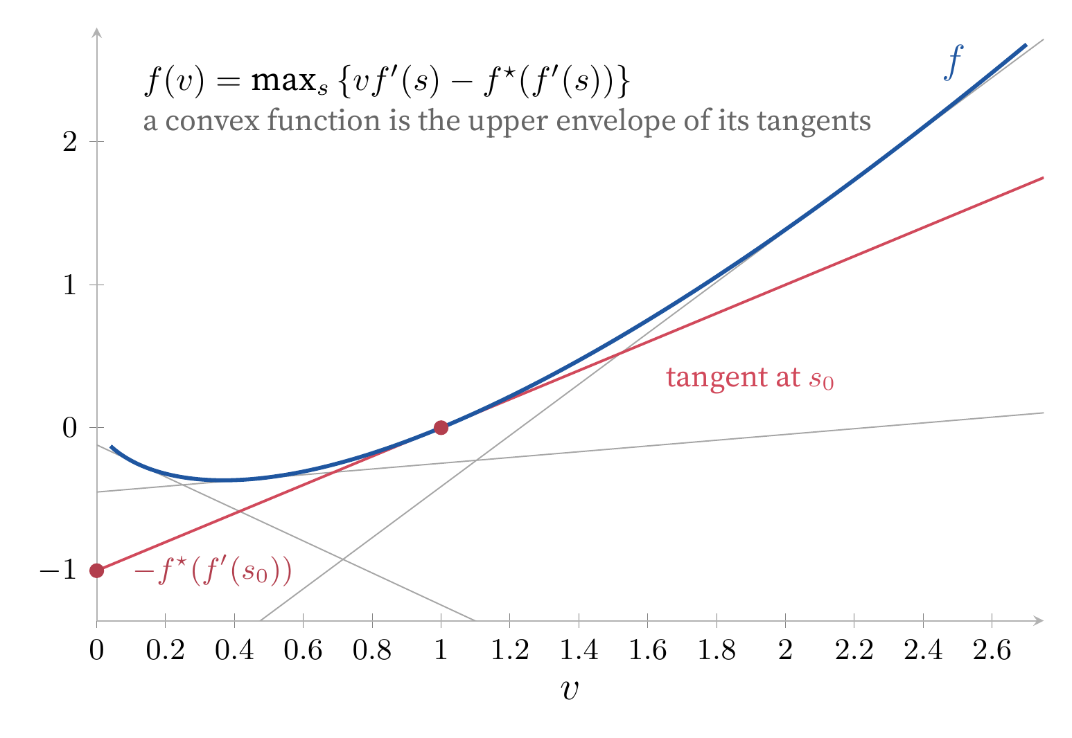
The variational representation. A differentiable, strictly convex f is the upper envelope of its tangent lines; the tangent with slope f′(s₀) has intercept −f⋆(f′(s₀)), and maximizing over tangents recovers f.
A second proof: the heat equation
There is a second route to the impossibility, with a complementary scope. The level-set argument in the main text rules out every scalar loss but needs mixtures in the family; this one stays inside the Gaussian family, where mixtures are unavailable, and rules out the classification recipe specifically. What it excludes is a utility $u$ and a strictly increasing readout $h$ satisfying $\mathbb{E}_{y \sim \mathcal{N}(\mu, \sigma^2)}[u(y)] = h(\mu + \sqrt{\beta}\,\sigma)$ on the whole half-plane, which is the form any variant of the recipe would have to take. Write $g(\mu, t) \triangleq \mathbb{E}_{y \sim \mathcal{N}(\mu, t)}[u(y)]$ with $t \triangleq \sigma^2$. As a convolution of $u$ with the Gaussian kernel, $g$ solves
$$ \frac{\partial g}{\partial t} = \frac{1}{2} \frac{\partial^2 g}{\partial \mu^2}. $$Substituting the hypothesis $g = h(s)$ with $s = \mu + \sqrt{\beta}\sqrt{t}$, the two sides become $\sqrt{\beta}\,h'(s) / (2\sigma) = h''(s) / 2$. Fix $s$ and vary $\sigma$ (adjusting $\mu = s - \sqrt{\beta}\,\sigma$ to keep $s$ constant). The right-hand side does not move. The left-hand side scales as $1/\sigma$. The only escape is $h'(s) = 0$ at every $s$: the readout is constant, and a constant acquisition function ranks nothing. (At $\beta = 0$ the argument relents exactly as it should: the equation forces $h'' = 0$, an affine readout of $\mu$, and the mean is elicitable.)
![Expected utilities are heat evolutions. g(μ, σ²) = E[u] under N(μ, σ²) starts at the step utility u = 𝟙(y > τ) and diffuses as σ grows. The proof says no such evolution is constant along the lines μ + √β σ = s unless it is constant everywhere.](/posts/likelihood-free-ucb/figures/heat-smoothing.png)
Expected utilities are heat evolutions. g(μ, σ²) = E[u] under N(μ, σ²) starts at the step utility u = 𝟙(y > τ) and diffuses as σ grows. The proof says no such evolution is constant along the lines μ + √β σ = s unless it is constant everywhere.
What classification can reach
The LFBO family is not barren of optimism. Take $u(y) = e^{ky}$: its expectation under $\mathcal{N}(\mu, \sigma^2)$ is $e^{k\mu + k^2\sigma^2/2}$, strictly increasing in $\mu + \tfrac{k}{2}\sigma^2$, the entropic risk measure. This is a genuine mean-plus-spread acquisition sitting inside the recipe. What the impossibility forbids is specifically the scale-equivariant kind: double the units of $y$ and $\sqrt{\beta}\,\sigma$ doubles along with $\mu$, while $\tfrac{k}{2}\sigma^2$ does not ($k$ carries units of $1/y$, so the exponential utility must be re-tuned whenever the outputs are rescaled). Variance-style optimism is available. Standard-deviation-style optimism is what cannot be had.
There is also an escape through higher dimension. The pair $(\mathbb{E}[y], \mathbb{E}[y^2])$ is jointly elicitable (by squared losses on each component), and $z_1 + \sqrt{\beta}\sqrt{z_2 - z_1^2}$ is a readout: the two-headed heteroscedastic regressor practitioners already fit.10 What the main text’s impossibility kills is a single output. Two outputs, estimating the first two moments separately, escape by the same route that makes expected shortfall elicitable in a pair with VaR.
What the marginal cannot see
The acquisition functions in the main text share a premise: each is a functional of the predictive distribution at a single point. PI, EI, UCB, the quantile — all ask what $p(y \mid \mathbf{x})$ says about $\mathbf{x}$ and nothing else. That is the precondition for the likelihood-free program, because raw pairs $(\mathbf{x}_i, y_i)$ are samples from exactly those marginals.
The rest of the acquisition zoo lives on the other side of that line. The knowledge gradient11 scores an observation by how much it improves the maximum of the posterior mean over the whole domain; entropy search and its descendants12 score it by the mutual information between $y(\mathbf{x})$ and the location or value of the global optimum. These are functionals of the posterior over $f$, the joint object with its correlation structure, rather than of any single marginal. For these acquisitions the likelihood-free wall is not elicitability but ontology: there is no loss to design, because the quantity being scored does not exist until a posterior is posited.
What the marginal world retains are the residues. Sever every cross-input correlation in the posterior, so that observing $y(\mathbf{x})$ informs only $\mathbf{x}$ itself, and the knowledge gradient collapses to $\mathbb{E}[\max(m(y) - \mu^{\ast}, 0)]$: expected improvement, computed on the distribution of the updated mean. Sever the same correlations in Thompson sampling, so that each candidate’s value is drawn from its marginal rather than from one function draw, and you get independent Thompson sampling: the variant the main text dismantles. The adjective was doing the work all along.
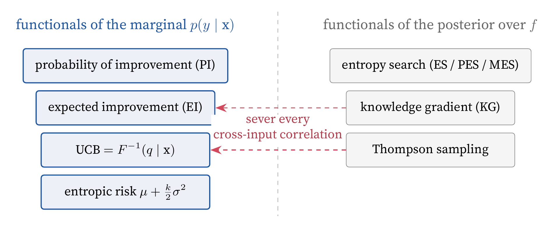
The dividing line. PI, EI, UCB, and the entropic score are functionals of the marginal p(y | x); knowledge gradient, entropy search, and Thompson sampling are functionals of the posterior over f. Severing every cross-input correlation sends KG to EI and Thompson sampling to its independent variant, which the main text collapses onto UCB. Entropy search leaves no marginal residue.
Srinivas, N., Krause, A., Kakade, S., & Seeger, M. (2010). Gaussian Process Optimization in the Bandit Setting: No Regret and Experimental Design. In Proceedings of the 27th International Conference on Machine Learning (ICML). ↩︎
Tiao, L. C., Klein, A., Seeger, M. W., Bonilla, E. V., Archambeau, C., & Ramos, F. (2021). BORE: Bayesian Optimization by Density-Ratio Estimation. In Proceedings of the 38th International Conference on Machine Learning (ICML). ↩︎
Song, J., Yu, L., Neiswanger, W., & Ermon, S. (2022). A General Recipe for Likelihood-Free Bayesian Optimization. In Proceedings of the 39th International Conference on Machine Learning (ICML). ↩︎
Salinas, D., Golebiowski, J., Klein, A., Seeger, M., & Archambeau, C. (2023). Optimizing Hyperparameters with Conformal Quantile Regression. In Proceedings of the 40th International Conference on Machine Learning (ICML). ↩︎
Wilson, J. T., Hutter, F., & Deisenroth, M. P. (2018). Maximizing Acquisition Functions for Bayesian Optimization. In Advances in Neural Information Processing Systems 31 (NeurIPS). ↩︎
Gneiting, T. (2011). Making and Evaluating Point Forecasts. Journal of the American Statistical Association, 106(494), 746–762. The convex-level-sets condition is due to K. Osband’s 1985 PhD thesis, Providing Incentives for Better Cost Forecasting (UC Berkeley). ↩︎
Romano, Y., Patterson, E., & Candès, E. (2019). Conformalized Quantile Regression. In Advances in Neural Information Processing Systems 32 (NeurIPS). ↩︎
The engineering arrivals are documented. ACHO (Doyle, 2022) guides conformal HPO by maximizing a conformalized upper quantile, the fixed-level rule adopted as a heuristic, and its follow-up (Doyle, 2025) benchmarks that rule alongside the Thompson sampling of Salinas et al. The derivation above upgrades the heuristic to the unique elicitable form of UCB, with the level pinned by $\beta$. ↩︎
The derivation follows the presentation in Chapter 5 of my PhD thesis, which rederives LFBO from the variational representation underlying $f$-divergence estimation. ↩︎
Fissler, T., & Ziegel, J. F. (2016). Higher Order Elicitability and Osband’s Principle. The Annals of Statistics, 44(4), 1680–1707. ↩︎
Frazier, P. I. (2018). A Tutorial on Bayesian Optimization. arXiv:1807.02811. Section 4.2 covers the knowledge gradient and its relationship to EI. ↩︎
Hennig, P., & Schuler, C. J. (2012). Entropy Search for Information-Efficient Global Optimization. JMLR, 13. Hernández-Lobato, J. M., Hoffman, M. W., & Ghahramani, Z. (2014). Predictive Entropy Search. In NeurIPS 27. Wang, Z., & Jegelka, S. (2017). Max-value Entropy Search. In ICML 34. ↩︎
