Exploring the Binance API in Python - Part II: Recent and Historical Trades
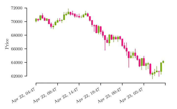
Table of Contents
Latest Price
Get the price at which the latest trade was executed:
r = s.get("https://api.binance.com/api/v3/ticker/price", params=dict(symbol="ETHAUD"))
The content of r.json():
{
  "price": "3032.17000000",
  "symbol": "ETHAUD"
}
Average Price
Get the average price of trades in the last 5 minutes:
r = s.get("https://api.binance.com/api/v3/avgPrice", params=dict(symbol="ETHAUD"))
The content of r.json():
{
  "mins": 5,
  "price": "3038.63364133"
}
Recent Trades
Get details of the most recent trades.
r = s.get("https://api.binance.com/api/v3/trades",
          params=dict(symbol="ETHAUD", limit=500))
block = r.json()
This returns a list of dictionaries that contain details of the trade.
[
  {
    "id": 909049,
    "isBestMatch": true,
    "isBuyerMaker": false,
    "price": "3041.05000000",
    "qty": "0.68053000",
    "quoteQty": "2069.52575650",
    "time": 1619205370059
  },
  {
    "id": 909050,
    "isBestMatch": true,
    "isBuyerMaker": true,
    "price": "3034.11000000",
    "qty": "0.67985000",
    "quoteQty": "2062.73968350",
    "time": 1619205476103
  }
  (...)
]
>>> data = create_trades_frame(block)
where
def create_trades_frame(trades):

    frame = pd.DataFrame(trades) \
        .assign(time=lambda trade: pd.to_datetime(trade.time, unit="ms"),
                price=lambda trade: pd.to_numeric(trade.price),
                qty=lambda trade: pd.to_numeric(trade.qty),
                quoteQty=lambda trade: pd.to_numeric(trade.quoteQty))
    return frame
| time | id | price | qty | quoteQty | isBuyerMaker | isBestMatch |
|---|---|---|---|---|---|---|
| 2021-04-23 17:39:09.812000 | 908551 | 2970.99 | 1.73541 | 5155.89 | False | True |
| 2021-04-23 17:39:13.854000 | 908552 | 2967.27 | 1.36668 | 4055.31 | False | True |
| 2021-04-23 17:39:15.059000 | 908553 | 2966.34 | 0.00941 | 27.9133 | True | True |
| 2021-04-23 17:39:16.948000 | 908554 | 2965.44 | 0.33998 | 1008.19 | False | True |
| 2021-04-23 17:39:16.949000 | 908555 | 2965.44 | 0.90989 | 2698.22 | False | True |
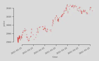
Scatter plot
sns.scatterplot(x="time", y="price", marker="+", data=data)
Historical Trades
num_blocks = 100
limit = 500

blocks = []
blocks.append(block)
for i in range(num_blocks):
    from_id = block[0]["id"] - limit  # get first trade of previous block
    r = s.get("https://api.binance.com/api/v3/historicalTrades",
              params=dict(symbol="ETHAUD", limit=limit, fromId=from_id))
    block = r.json()
    blocks.append(block)
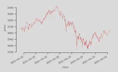
Let us chain together these blocks of trades. In other words, we wish to convert this list of blocks, where each block contains a list of trades, into a single “flat” list of trades.
>>> data = create_trades_frame(chain(*blocks))
where we import the chain function from itertools:
from itertools import chain
Scatter plot
sns.scatterplot(x="time", y="price", marker="x", s=0.5, alpha=0.2, data=data)
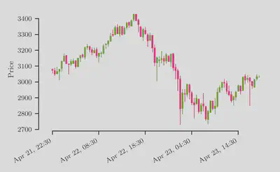
Open-High-Low-Close (OHLC) Data
data_ohlc = data.set_index("time").price.resample("30T").ohlc()
| time | open | high | low | close |
|---|---|---|---|---|
| 2021-04-21 22:30:00 | 3079.11 | 3085.95 | 3055 | 3074.12 |
| 2021-04-21 23:00:00 | 3071.99 | 3089.71 | 3039.44 | 3049.73 |
| 2021-04-21 23:30:00 | 3052.51 | 3096.03 | 3052.51 | 3065.93 |
| 2021-04-22 00:00:00 | 3066.54 | 3084.58 | 3012.32 | 3080.94 |
| 2021-04-22 00:30:00 | 3084.04 | 3133.27 | 3064.27 | 3132.16 |
Candlestick chart
mpf.plot(data_ohlc, type="candle", style="binance")
Volume Data
series_volume = data.set_index("time").quoteQty.resample("30T").sum()
Concatentate this together with the OHLC DataFrame:
frame = data_ohlc.assign(volume=series_volume)
| time | open | high | low | close | volume |
|---|---|---|---|---|---|
| 2021-04-21 22:30:00 | 3079.11 | 3085.95 | 3055 | 3074.12 | 643973 |
| 2021-04-21 23:00:00 | 3071.99 | 3089.71 | 3039.44 | 3049.73 | 848766 |
| 2021-04-21 23:30:00 | 3052.51 | 3096.03 | 3052.51 | 3065.93 | 363078 |
| 2021-04-22 00:00:00 | 3066.54 | 3084.58 | 3012.32 | 3080.94 | 1.18854e+06 |
| 2021-04-22 00:30:00 | 3084.04 | 3133.27 | 3064.27 | 3132.16 | 901508 |
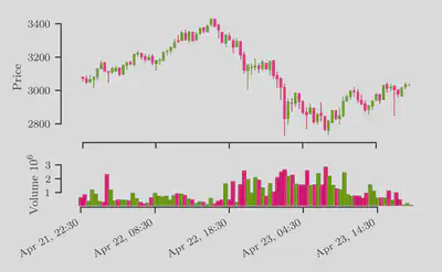
Candlestick chart with volume
fig, (ax1, ax2) = plt.subplots(nrows=2, gridspec_kw=dict(height_ratios=[3, 1]))

mpf.plot(frame, type="candle", style="binance", volume=ax2, ax=ax1)
fig.autofmt_xdate()

plt.show()
Candlestick
We can also obtain summarize the data into a format suitable candlestick chart at server-side by directly calling the following endpoint:
r = s.get("https://api.binance.com/api/v3/klines",
          params=dict(symbol="ETHAUD", interval="4h"))

frame = pd.DataFrame(data=r.json(),
                     columns=["open_time",
                              "open",
                              "high",
                              "low",
                              "close",
                              "volume",
                              "close_time",
                              "quote_asset_volume",
                              "number_of_trades",
                              "taker_buy_base_asset_volume",
                              "taker_buy_quote_asset_volume",
                              "ignore"], dtype="float64") \
          .assign(open_time=lambda interval: pd.to_datetime(interval.open_time, unit="ms"),
                  close_time=lambda interval: pd.to_datetime(interval.close_time, unit="ms")) \
          .set_index("close_time")

If you don’t require fine-grained data on every single trade, then this might be more appropriate.
Links and Further Readings
- Blog posts:
- The first post in this series: Exploring the Binance API in Python - Part I: The Order Book
To receive updates on more posts like this, follow me on Twitter and GitHub!
Appendix
I - Import statements
import requests

import numpy as np
import pandas as pd

import matplotlib.pyplot as plt
import mplfinance as mpf
import seaborn as sns