Exploring the Binance API in Python - Part I: The Order Book
In this post, we will explore the live order book data on Binance through its official API using Python.
We directly interact with the API endpoints and explicitly make the low-level HTTP requests ourselves. If you’re just looking for a high-level way to interact with the API endpoints that abstracts away these details please check out python-binance, an unofficial, but slick and well-designed Python Client for the Binance API.
We will be making the requests using the requests library. Thereafter, we will process the results with pandas, and visualize them with matplotlib and seaborn. Let’s import these dependencies now:
import requests
import pandas as pd
import matplotlib.pyplot as plt
import seaborn as sns
To make a GET request for the symbol ETHBUSD from the /depth endpoint:
r = requests.get("https://api.binance.com/api/v3/depth",
                 params=dict(symbol="ETHBUSD"))
results = r.json()
Load the buy and sell orders, or bids and asks, into respective DataFrames:
frames = {side: pd.DataFrame(data=results[side], columns=["price", "quantity"],
                             dtype=float)
          for side in ["bids", "asks"]}
Concatenate the DataFrames containing bids and asks into one big frame:
frames_list = [frames[side].assign(side=side) for side in frames]
data = pd.concat(frames_list, axis="index",
                 ignore_index=True, sort=True)
Get a statistical summary of the price levels in the bids and asks:
price_summary = data.groupby("side").price.describe()
price_summary.to_markdown()
| side | count | mean | std | min | 25% | 50% | 75% | max |
|---|---|---|---|---|---|---|---|---|
| asks | 100 | 1057.86 | 0.696146 | 1056.64 | 1057.2 | 1057.91 | 1058.49 | 1059.04 |
| bids | 100 | 1055.06 | 0.832385 | 1053.7 | 1054.4 | 1054.85 | 1055.82 | 1056.58 |
Note that the Binance API only provides the lowest 100 asks
and the highest 100 bids (see the count column).
Top of the book
The prices of the most recent trades will be somewhere between the maximum bid price and the minimum asking price. This is known as the top of the book. The difference between these two price levels is known as the bid-ask spread.
>>> frames["bids"].price.max()
1056.58
>>> frames["asks"].price.min()
1056.64
We can also get this information from the /ticker/bookTicker endpoint:
r = requests.get("https://api.binance.com/api/v3/ticker/bookTicker", params=dict(symbol="ETHBUSD"))
book_top = r.json()
Read this into a Pandas Series and render as a Markdown table:
name = book_top.pop("symbol")  # get symbol and also delete at the same time
s = pd.Series(book_top, name=name, dtype=float)
s.to_markdown()
| ETHBUSD | |
|---|---|
| bidPrice | 1056.58 |
| bidQty | 7.555 |
| askPrice | 1056.64 |
| askQty | 7.43152 |
Scatter plot
Let us visualize all the order book entries using a scatter plot, showing price along the $x$-axis, and quantity along the $y$-axis. The hue signifies whether the entry is an “ask” or a “bid”.
fig, ax = plt.subplots()

ax.set_title(f"Last update: {t} (ID: {last_update_id})")

sns.scatterplot(x="price", y="quantity", hue="side", data=data, ax=ax)

ax.set_xlabel("Price")
ax.set_ylabel("Quantity")

plt.show()
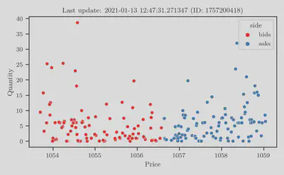
This is the most verbose visualization, displaying all the raw information, but perhaps also providing the least amount of actionable insights.
Histogram plot
We can compress this information into a histogram plot.
fig, ax = plt.subplots()

ax.set_title(f"Last update: {t} (ID: {last_update_id})")

sns.histplot(x="price", hue="side", binwidth=binwidth, data=data, ax=ax)
sns.rugplot(x="price", hue="side", data=data, ax=ax)

plt.show()
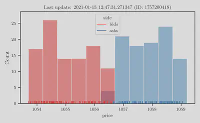
This shows the number of bids or asks at specific price points, but obscures the volume (or quantity).
This is obviously misleading. For example, there could be 1 bid at price $p_1$ and and 100 bids at $p_2$. However, the 1 bid at price $p_1$ could be for 100 ETH, while each of those 100 bids at $p_2$ could be for just 1 ETH. At both price points, the total quantity of ETH being bid is in fact identical. Yet this plot would suggest that there is 100 times greater demand for ETH at $p_2$.
Weighted histogram plot
This is easy to fix, simply by weighting each entry by the quantity.
This just amounts to setting weights="quantity":
fig, ax = plt.subplots()

ax.set_title(f"Last update: {t} (ID: {last_update_id})")

sns.histplot(x="price", weights="quantity", hue="side", binwidth=binwidth, data=data, ax=ax)
sns.scatterplot(x="price", y="quantity", hue="side", data=data, ax=ax)

ax.set_xlabel("Price")
ax.set_ylabel("Quantity")

plt.show()
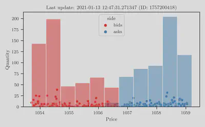
This paints a more accurate picture about supply-and-demand, but still offers limited actionable insights.
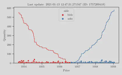
Weighted empirical CDF (ECDF) plot – aka the “Depth Chart”
Now we finally arrive at the depth chart, which is a popular visualization that is ubiquitous across exchanges and trading platforms. The depth chart is essentially just a combination of two empirical cumulative distribution function (CDF), or ECDF, plots.
More precisely, they are weighted and unnormalized ECDF plots. As before, they are weighted by the quantity and are unnormalized in the sense that they are not proportions between $[0, 1]$. Rather, they are simply kept as counts. Additionally, in the case of bids, we take the complementary ECDF (which basically reverses the order in which the cumulative sum is taken).
In code, this amounts to making calls to sns.ecdfplot with the options
weights="quantity" (self-explanatory) and stat="count" (to keep the plot
unnormalized). Finally, for the bids, we add the option complementary=True.
Putting it all together:
fig, ax = plt.subplots()

ax.set_title(f"Last update: {t} (ID: {last_update_id})")

sns.ecdfplot(x="price", weights="quantity", stat="count", complementary=True, data=frames["bids"], ax=ax)
sns.ecdfplot(x="price", weights="quantity", stat="count", data=frames["asks"], ax=ax)
sns.scatterplot(x="price", y="quantity", hue="side", data=data, ax=ax)

ax.set_xlabel("Price")
ax.set_ylabel("Quantity")

plt.show()
To receive updates on more posts like this, follow me on Twitter and GitHub!